手把手教你在Python中实现文本分类（附代码、数据集）_文本分词 i

#导入数据集预处理、特征工程和模型训练所需的库
from sklearn import model_selection, preprocessing, linear_model, naive_bayes, metrics, svm
from sklearn.feature_extraction.text import TfidfVectorizer, CountVectorizer
from sklearn import decomposition, ensemble

import pandas, xgboost, numpy, textblob, string
from keras.preprocessing import text, sequence
from keras import layers, models, optimizers

一、准备数据集


在本文中，我使用亚马逊的评论数据集，它可以从这个链接下载：



> 
> [https://gist.github.com/kunalj101/ad1d9c58d338e20d09ff26bcc06c4235](https://bbs.csdn.net/topics/618317507)
> 


这个数据集包含3.6M的文本评论内容及其标签，我们只使用其中一小部分数据。首先，将下载的数据加载到包含两个列（文本和标签）的pandas的数据结构（dataframe）中。


数据集链接：



> 
> [https://drive.google.com/drive/folders/0Bz8a\_Dbh9Qhbfll6bVpmNUtUcFdjYmF2SEpmZUZUcVNiMUw1TWN6RDV3a0JHT3kxLVhVR2M](https://bbs.csdn.net/topics/618317507)
> 

#加载数据集
data = open(‘data/corpus’).read()
labels, texts = [], []
for i, line in enumerate(data.split(“\n”)):
content = line.split()
labels.append(content[0])
texts.append(content[1])

#创建一个dataframe，列名为text和label
trainDF = pandas.DataFrame()
trainDF[‘text’] = texts
trainDF[‘label’] = labels

接下来，我们将数据集分为训练集和验证集，这样我们可以训练和测试分类器。另外，我们将编码我们的目标列，以便它可以在机器学习模型中使用:

#将数据集分为训练集和验证集
train_x, valid_x, train_y, valid_y = model_selection.train_test_split(trainDF[‘text’], trainDF[‘label’])

label编码为目标变量

encoder = preprocessing.LabelEncoder()
train_y = encoder.fit_transform(train_y)
valid_y = encoder.fit_transform(valid_y)

二、特征工程


接下来是特征工程，在这一步，原始数据将被转换为特征向量，另外也会根据现有的数据创建新的特征。为了从数据集中选出重要的特征，有以下几种方式：


* 计数向量作为特征
* TF-IDF向量作为特征
	+ 单个词语级别
	+ 多个词语级别（N-Gram）
	+ 词性级别
* 词嵌入作为特征
* 基于文本/NLP的特征
* 主题模型作为特征


接下来分别看看它们如何实现：


2.1 计数向量作为特征


计数向量是数据集的矩阵表示，其中每行代表来自语料库的文档，每列表示来自语料库的术语，并且每个单元格表示特定文档中特定术语的频率计数：

#创建一个向量计数器对象
count_vect = CountVectorizer(analyzer=‘word’, token_pattern=r’\w{1,}')
count_vect.fit(trainDF[‘text’])

#使用向量计数器对象转换训练集和验证集
xtrain_count = count_vect.transform(train_x)
xvalid_count = count_vect.transform(valid_x)

2.2 TF-IDF向量作为特征


TF-IDF的分数代表了词语在文档和整个语料库中的相对重要性。TF-IDF分数由两部分组成：第一部分是计算标准的词语频率（TF），第二部分是逆文档频率（IDF）。其中计算语料库中文档总数除以含有该词语的文档数量，然后再取对数就是逆文档频率。


TF(t)=（该词语在文档出现的次数）/（文档中词语的总数）


IDF(t)= log\_e（文档总数/出现该词语的文档总数）


TF-IDF向量可以由不同级别的分词产生（单个词语，词性，多个词（n-grams））


* 词语级别TF-IDF：矩阵代表了每个词语在不同文档中的TF-IDF分数。
* N-gram级别TF-IDF: N-grams是多个词语在一起的组合，这个矩阵代表了N-grams的TF-IDF分数。
* 词性级别TF-IDF：矩阵代表了语料中多个词性的TF-IDF分数。
* * ```
#词语级tf-idf
tfidf_vect = TfidfVectorizer(analyzer='word', token_pattern=r'\w{1,}', max_features=5000)
tfidf_vect.fit(trainDF['text'])
xtrain_tfidf =  tfidf_vect.transform(train_x)
xvalid_tfidf =  tfidf_vect.transform(valid_x)

# ngram 级tf-idf
tfidf_vect_ngram = TfidfVectorizer(analyzer='word', token_pattern=r'\w{1,}', ngram_range=(2,3), max_features=5000)
tfidf_vect_ngram.fit(trainDF['text'])
xtrain_tfidf_ngram =  tfidf_vect_ngram.transform(train_x)
xvalid_tfidf_ngram =  tfidf_vect_ngram.transform(valid_x)

#词性级tf-idf
tfidf_vect_ngram_chars = TfidfVectorizer(analyzer='char', token_pattern=r'\w{1,}', ngram_range=(2,3), max_features=5000)
tfidf_vect_ngram_chars.fit(trainDF['text'])
xtrain_tfidf_ngram_chars =  tfidf_vect_ngram_chars.transform(train_x)
xvalid_tfidf_ngram_chars =  tfidf_vect_ngram_chars.transform(valid_x)

2.3 词嵌入

词嵌入是使用稠密向量代表词语和文档的一种形式。向量空间中单词的位置是从该单词在文本中的上下文学习到的，词嵌入可以使用输入语料本身训练，也可以使用预先训练好的词嵌入模型生成，词嵌入模型有：Glove, FastText,Word2Vec。它们都可以下载，并用迁移学习的方式使用。想了解更多的词嵌入资料，可以访问：

https://www.analyticsvidhya.com/blog/2017/06/word-embeddings-count-word2veec/

接下来介绍如何在模型中使用预先训练好的词嵌入模型，主要有四步：

1. 加载预先训练好的词嵌入模型

2. 创建一个分词对象

3. 将文本文档转换为分词序列并填充它们

4. 创建分词和各自嵌入的映射

#加载预先训练好的词嵌入向量
embeddings_index = {}
for i, line in enumerate(open('data/wiki-news-300d-1M.vec')):
values = line.split()
embeddings_index[values[0]] = numpy.asarray(values[1:], dtype='float32')

#创建一个分词器
token = text.Tokenizer()
token.fit_on_texts(trainDF['text'])
word_index = token.word_index

#将文本转换为分词序列，并填充它们保证得到相同长度的向量
train_seq_x = sequence.pad_sequences(token.texts_to_sequences(train_x), maxlen=70)
valid_seq_x = sequence.pad_sequences(token.texts_to_sequences(valid_x), maxlen=70)

#创建分词嵌入映射
embedding_matrix = numpy.zeros((len(word_index) + 1, 300))
for word, i in word_index.items():
embedding_vector = embeddings_index.get(word)
if embedding_vector is not None:
embedding_matrix[i] = embedding_vector

2.4 基于文本/NLP的特征

创建许多额外基于文本的特征有时可以提升模型效果。比如下面的例子：

• 文档的词语计数—文档中词语的总数量
• 文档的词性计数—文档中词性的总数量
• 文档的平均字密度–文件中使用的单词的平均长度
• 完整文章中的标点符号出现次数–文档中标点符号的总数量
• 整篇文章中的大写次数—文档中大写单词的数量
• 完整文章中标题出现的次数—文档中适当的主题（标题）的总数量
• 词性标注的频率分布
  • 名词数量
  • 动词数量
  • 形容词数量
  • 副词数量
  • 代词数量

这些特征有很强的实验性质，应该具体问题具体分析。

trainDF['char_count'] = trainDF['text'].apply(len)
trainDF['word_count'] = trainDF['text'].apply(lambda x: len(x.split()))
trainDF['word_density'] = trainDF['char_count'] / (trainDF['word_count']+1)
trainDF['punctuation_count'] = trainDF['text'].apply(lambda x: len("".join(_ for _ in x if _ in string.punctuation)))
trainDF['title_word_count'] = trainDF['text'].apply(lambda x: len([wrd for wrd in x.split() if wrd.istitle()]))
trainDF['upper_case_word_count'] = trainDF['text'].apply(lambda x: len([wrd for wrd in x.split() if wrd.isupper()]))

trainDF['char_count'] = trainDF['text'].apply(len)
trainDF['word_count'] = trainDF['text'].apply(lambda x: len(x.split()))
trainDF['word_density'] = trainDF['char_count'] / (trainDF['word_count']+1)
trainDF['punctuation_count'] = trainDF['text'].apply(lambda x: len("".join(_ for _ in x if _ in string.punctuation)))
trainDF['title_word_count'] = trainDF['text'].apply(lambda x: len([wrd for wrd in x.split() if wrd.istitle()]))
trainDF['upper_case_word_count'] = trainDF['text'].apply(lambda x: len([wrd for wrd in x.split() if wrd.isupper()]))
pos_family = {
'noun' : ['NN','NNS','NNP','NNPS'],
'pron' : ['PRP','PRP$','WP','WP$'],
'verb' : ['VB','VBD','VBG','VBN','VBP','VBZ'],
'adj' :  ['JJ','JJR','JJS'],
'adv' : ['RB','RBR','RBS','WRB']
}

#检查和获得特定句子中的单词的词性标签数量
def check_pos_tag(x, flag):
cnt = 0
try:
wiki = textblob.TextBlob(x)
for tup in wiki.tags:
ppo = list(tup)[1]
if ppo in pos_family[flag]:
cnt += 1
except:
pass
return cnt

trainDF['noun_count'] = trainDF['text'].apply(lambda x: check_pos_tag(x, 'noun'))
trainDF['verb_count'] = trainDF['text'].apply(lambda x: check_pos_tag(x, 'verb'))
trainDF['adj_count'] = trainDF['text'].apply(lambda x: check_pos_tag(x, 'adj'))
trainDF['adv_count'] = trainDF['text'].apply(lambda x: check_pos_tag(x, 'adv'))
trainDF['pron_count'] = trainDF['text'].apply(lambda x: check_pos_tag(x, 'pron'))

2.5 主题模型作为特征

主题模型是从包含重要信息的文档集中识别词组（主题）的技术，我已经使用LDA生成主题模型特征。LDA是一个从固定数量的主题开始的迭代模型，每一个主题代表了词语的分布，每一个文档表示了主题的分布。虽然分词本身没有意义，但是由主题表达出的词语的概率分布可以传达文档思想。如果想了解更多主题模型，请访问：

https://www.analyticsvidhya.com/blog/2016/08/beginners-guide-to-topic-modeling-in-python/

我们看看主题模型运行过程：

#训练主题模型
lda_model = decomposition.LatentDirichletAllocation(n_components=20, learning_method='online', max_iter=20)
X_topics = lda_model.fit_transform(xtrain_count)
topic_word = lda_model.components_
vocab = count_vect.get_feature_names()

#可视化主题模型
n_top_words = 10
topic_summaries = []
for i, topic_dist in enumerate(topic_word):
topic_words = numpy.array(vocab)[numpy.argsort(topic_dist)][:-(n_top_words+1):-1]
topic_summaries.append(' '.join(topic_words)

三、建模

文本分类框架的最后一步是利用之前创建的特征训练一个分类器。关于这个最终的模型，机器学习中有很多模型可供选择。我们将使用下面不同的分类器来做文本分类：

• 朴素贝叶斯分类器
• 线性分类器
• 支持向量机（SVM）
• Bagging Models
• Boosting Models
• 浅层神经网络
• 深层神经网络
  • 卷积神经网络（CNN）
  • LSTM
  • GRU
  • 双向RNN
  • 循环卷积神经网络（RCNN）
  • 其它深层神经网络的变种

接下来我们详细介绍并使用这些模型。下面的函数是训练模型的通用函数，它的输入是分类器、训练数据的特征向量、训练数据的标签，验证数据的特征向量。我们使用这些输入训练一个模型，并计算准确度。

def train_model(classifier, feature_vector_train, label, feature_vector_valid, is_neural_net=False):
# fit the training dataset on the classifier
classifier.fit(feature_vector_train, label)

# predict the labels on validation dataset
predictions = classifier.predict(feature_vector_valid)

if is_neural_net:
predictions = predictions.argmax(axis=-1)

return metrics.accuracy_score(predictions, valid_y)

3.1 朴素贝叶斯

利用sklearn框架，在不同的特征下实现朴素贝叶斯模型。

朴素贝叶斯是一种基于贝叶斯定理的分类技术，并且假设预测变量是独立的。朴素贝叶斯分类器假设一个类别中的特定特征与其它存在的特征没有任何关系。

想了解朴素贝叶斯算法细节可点击：

A Naive Bayes classifier assumes that the presence of a particular feature in a class is unrelated to the presence of any other feature

#特征为计数向量的朴素贝叶斯
accuracy = train_model(naive_bayes.MultinomialNB(), xtrain_count, train_y, xvalid_count)
print "NB, Count Vectors: ", accuracy

#特征为词语级别TF-IDF向量的朴素贝叶斯
accuracy = train_model(naive_bayes.MultinomialNB(), xtrain_tfidf, train_y, xvalid_tfidf)
print "NB, WordLevel TF-IDF: ", accuracy

#特征为多个词语级别TF-IDF向量的朴素贝叶斯
accuracy = train_model(naive_bayes.MultinomialNB(), xtrain_tfidf_ngram, train_y, xvalid_tfidf_ngram)
print "NB, N-Gram Vectors: ", accuracy

#特征为词性级别TF-IDF向量的朴素贝叶斯
accuracy = train_model(naive_bayes.MultinomialNB(), xtrain_tfidf_ngram_chars, train_y, xvalid_tfidf_ngram_chars)
print "NB, CharLevel Vectors: ", accuracy
#输出结果
NB, Count Vectors:  0.7004
NB, WordLevel TF-IDF:  0.7024
NB, N-Gram Vectors:  0.5344
NB, CharLevel Vectors:  0.6872

3.2 线性分类器

实现一个线性分类器（Logistic Regression）：Logistic回归通过使用logistic / sigmoid函数估计概率来度量类别因变量与一个或多个独立变量之间的关系。如果想了解更多关于logistic回归，请访问：

https://www.analyticsvidhya.com/blog/2015/10/basics-logistic-regression/

# Linear Classifier on Count Vectors
accuracy = train_model(linear_model.LogisticRegression(), xtrain_count, train_y, xvalid_count)
print "LR, Count Vectors: ", accuracy

#特征为词语级别TF-IDF向量的线性分类器
accuracy = train_model(linear_model.LogisticRegression(), xtrain_tfidf, train_y, xvalid_tfidf)
print "LR, WordLevel TF-IDF: ", accuracy

#特征为多个词语级别TF-IDF向量的线性分类器
accuracy = train_model(linear_model.LogisticRegression(), xtrain_tfidf_ngram, train_y, xvalid_tfidf_ngram)
print "LR, N-Gram Vectors: ", accuracy

#特征为词性级别TF-IDF向量的线性分类器
accuracy = train_model(linear_model.LogisticRegression(), xtrain_tfidf_ngram_chars, train_y, xvalid_tfidf_ngram_chars)
print "LR, CharLevel Vectors: ", accuracy
#输出结果
LR, Count Vectors:  0.7048
LR, WordLevel TF-IDF:  0.7056
LR, N-Gram Vectors:  0.4896
LR, CharLevel Vectors:  0.7012

3.3 实现支持向量机模型

支持向量机（SVM）是监督学习算法的一种，它可以用来做分类或回归。该模型提取了分离两个类的最佳超平面或线。如果想了解更多关于SVM，请访问：

https://www.analyticsvidhya.com/blog/2017/09/understaing-support-vector-machine-example-code/

#特征为多个词语级别TF-IDF向量的SVM
accuracy = train_model(svm.SVC(), xtrain_tfidf_ngram, train_y, xvalid_tfidf_ngram)
print "SVM, N-Gram Vectors: ", accuracy
#输出结果
SVM, N-Gram Vectors:  0.5296

3.4 Bagging Model

实现一个随机森林模型：随机森林是一种集成模型，更准确地说是Bagging model。它是基于树模型家族的一部分。如果想了解更多关于随机森林，请访问：

https://www.analyticsvidhya.com/blog/2014/06/introduction-random-forest-simplified/

#特征为计数向量的RF

accuracy = train_model(ensemble.RandomForestClassifier(), xtrain_count, train_y, xvalid_count)

print "RF, Count Vectors: ", accuracy

#特征为词语级别TF-IDF向量的RF

accuracy = train_model(ensemble.RandomForestClassifier(), xtrain_tfidf, train_y, xvalid_tfidf)

print "RF, WordLevel TF-IDF: ", accuracy

#输出结果

RF, Count Vectors: 0.6972

RF, WordLevel TF-IDF: 0.6988

3.5 Boosting Model

实现一个Xgboost模型：Boosting model是另外一种基于树的集成模型。Boosting是一种机器学习集成元算法，主要用于减少模型的偏差，它是一组机器学习算法，可以把弱学习器提升为强学习器。其中弱学习器指的是与真实类别只有轻微相关的分类器（比随机猜测要好一点）。如果想了解更多，请访问：

https://www.analyticsvidhya.com/blog/2016/01/xgboost-algorithm-easy-steps/

#特征为计数向量的Xgboost

accuracy = train_model(xgboost.XGBClassifier(), xtrain_count.tocsc(), train_y, xvalid_count.tocsc())

print "Xgb, Count Vectors: ", accuracy

#特征为词语级别TF-IDF向量的Xgboost

accuracy = train_model(xgboost.XGBClassifier(), xtrain_tfidf.tocsc(), train_y, xvalid_tfidf.tocsc())

print "Xgb, WordLevel TF-IDF: ", accuracy

#特征为词性级别TF-IDF向量的Xgboost

accuracy = train_model(xgboost.XGBClassifier(), xtrain_tfidf_ngram_chars.tocsc(), train_y, xvalid_tfidf_ngram_chars.tocsc())

print "Xgb, CharLevel Vectors: ", accuracy

#输出结果

Xgb, Count Vectors: 0.6324

Xgb, WordLevel TF-IDF: 0.6364

Xgb, CharLevel Vectors: 0.6548

3.6 浅层神经网络

神经网络被设计成与生物神经元和神经系统类似的数学模型，这些模型用于发现被标注数据中存在的复杂模式和关系。一个浅层神经网络主要包含三层神经元-输入层、隐藏层、输出层。如果想了解更多关于浅层神经网络，请访问：

https://www.analyticsvidhya.com/blog/2017/05/neural-network-from-scratch-in-python-and-r/

def create_model_architecture(input_size):

create input layer

input_layer = layers.Input((input_size, ), sparse=True)

create hidden layer

hidden_layer = layers.Dense(100, activation=“relu”)(input_layer)

create output layer

output_layer = layers.Dense(1, activation=“sigmoid”)(hidden_layer)

classifier = models.Model(inputs = input_layer, outputs = output_layer)

classifier.compile(optimizer=optimizers.Adam(), loss=‘binary_crossentropy’)

return classifier

classifier = create_model_architecture(xtrain_tfidf_ngram.shape[1])

accuracy = train_model(classifier, xtrain_tfidf_ngram, train_y, xvalid_tfidf_ngram, is_neural_net=True)

print “NN, Ngram Level TF IDF Vectors”, accuracy

#输出结果：

Epoch 1/1

7500/7500 [==============================] - 1s 67us/step - loss: 0.6909

NN, Ngram Level TF IDF Vectors 0.5296

3.7 深层神经网络

深层神经网络是更复杂的神经网络，其中隐藏层执行比简单Sigmoid或Relu激活函数更复杂的操作。不同类型的深层学习模型都可以应用于文本分类问题。

• 卷积神经网络

卷积神经网络中，输入层上的卷积用来计算输出。本地连接结果中，每一个输入单元都会连接到输出神经元上。每一层网络都应用不同的滤波器（filter）并组合它们的结果。

如果想了解更多关于卷积神经网络，请访问：

https://www.analyticsvidhya.com/blog/2017/06/architecture-of-convolutional-neural-networks-simplified-demystified/

def create_cnn():

Add an Input Layer

input_layer = layers.Input((70, ))

Add the word embedding Layer

embedding_layer = layers.Embedding(len(word_index) + 1, 300, weights=[embedding_matrix], trainable=False)(input_layer)

embedding_layer = layers.SpatialDropout1D(0.3)(embedding_layer)

Add the convolutional Layer

conv_layer = layers.Convolution1D(100, 3, activation=“relu”)(embedding_layer)

Add the pooling Layer

pooling_layer = layers.GlobalMaxPool1D()(conv_layer)

Add the output Layers

output_layer1 = layers.Dense(50, activation=“relu”)(pooling_layer)

output_layer1 = layers.Dropout(0.25)(output_layer1)

output_layer2 = layers.Dense(1, activation=“sigmoid”)(output_layer1)

Compile the model

model = models.Model(inputs=input_layer, outputs=output_layer2)

model.compile(optimizer=optimizers.Adam(), loss=‘binary_crossentropy’)

return model

classifier = create_cnn()

accuracy = train_model(classifier, train_seq_x, train_y, valid_seq_x, is_neural_net=True)

print “CNN, Word Embeddings”, accuracy

#输出结果

Epoch 1/1

7500/7500 [==============================] - 12s 2ms/step - loss: 0.5847

CNN, Word Embeddings 0.5296

• 循环神经网络-LSTM

最后

Python崛起并且风靡，因为优点多、应用领域广、被大牛们认可。学习 Python 门槛很低，但它的晋级路线很多，通过它你能进入机器学习、数据挖掘、大数据，CS等更加高级的领域。Python可以做网络应用，可以做科学计算，数据分析，可以做网络爬虫，可以做机器学习、自然语言处理、可以写游戏、可以做桌面应用…Python可以做的很多，你需要学好基础，再选择明确的方向。这里给大家分享一份全套的 Python 学习资料，给那些想学习 Python 的小伙伴们一点帮助！

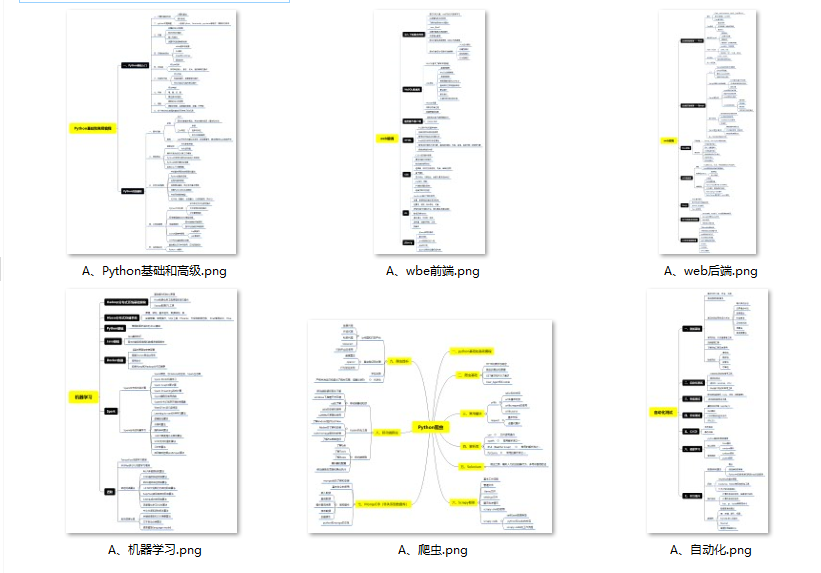
👉Python所有方向的学习路线👈

Python所有方向的技术点做的整理，形成各个领域的知识点汇总，它的用处就在于，你可以按照上面的知识点去找对应的学习资源，保证自己学得较为全面。

👉Python必备开发工具👈

工欲善其事必先利其器。学习Python常用的开发软件都在这里了，给大家节省了很多时间。

👉Python全套学习视频👈

我们在看视频学习的时候，不能光动眼动脑不动手，比较科学的学习方法是在理解之后运用它们，这时候练手项目就很适合了。

👉实战案例👈

学python就与学数学一样，是不能只看书不做题的，直接看步骤和答案会让人误以为自己全都掌握了，但是碰到生题的时候还是会一筹莫展。

因此在学习python的过程中一定要记得多动手写代码，教程只需要看一两遍即可。

👉大厂面试真题👈

我们学习Python必然是为了找到高薪的工作，下面这些面试题是来自阿里、腾讯、字节等一线互联网大厂最新的面试资料，并且有阿里大佬给出了权威的解答，刷完这一套面试资料相信大家都能找到满意的工作。

需要这份系统化学习资料的朋友，可以戳这里无偿获取

一个人可以走的很快，但一群人才能走的更远！不论你是正从事IT行业的老鸟或是对IT行业感兴趣的新人，都欢迎加入我们的的圈子（技术交流、学习资源、职场吐槽、大厂内推、面试辅导），让我们一起学习成长！