2024美赛B题深度剖析|详细建模+代码实现

首先回顾一下本次美赛B题：

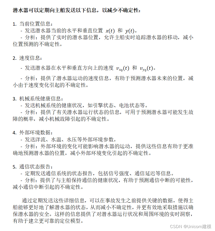
问题1的解决思路如下：

python示例代码：

import numpy as np
import matplotlib.pyplot as plt

# 模拟时间
time = np.linspace(0, 10, 100)

# 初始位置
x0, y0 = 0, 0

# 期望速度函数（可根据实际情况调整）
def expected_velocity(t):
    return np.sin(t)

# 不确定性项的标准差（可根据实际情况调整）
sigma_x = 0.1
sigma_y = 0.1

# 模拟机械故障和环境不确定性的随机项
delta_x = np.random.normal(0, sigma_x, len(time))
delta_y = np.random.normal(0, sigma_y, len(time))

# 计算位置
x = x0 + np.cumsum(expected_velocity(time) + delta_x)
y = y0 + np.cumsum(expected_velocity(time) + delta_y)

# 可视化模拟结果
plt.figure(figsize=(10, 6))
plt.plot(time, x, label='Simulated X Position')
plt.plot(time, y, label='Simulated Y Position')
plt.xlabel('Time')
plt.ylabel('Position')
plt.legend()
plt.title('Simulated Submarine Position Over Time')
plt.show()

matlab示例代码：

% 模拟时间
time = linspace(0, 10, 100);

% 初始位置
x0 = 0;
y0 = 0;

% 期望速度函数（可根据实际情况调整）
expected_velocity = @(t) sin(t);

% 不确定性项的标准差（可根据实际情况调整）
sigma_x = 0.1;
sigma_y = 0.1;

% 模拟机械故障和环境不确定性的随机项
delta_x = sigma_x * randn(size(time));
delta_y = sigma_y * randn(size(time));

% 计算位置
x = x0 + cumsum(expected_velocity(time) + delta_x);
y = y0 + cumsum(expected_velocity(time) + delta_y);

% 可视化模拟结果
figure;
plot(time, x, 'LineWidth', 1.5, 'DisplayName', 'Simulated X Position');
hold on;
plot(time, y, 'LineWidth', 1.5, 'DisplayName', 'Simulated Y Position');
xlabel('Time');
ylabel('Position');
legend('Location', 'Best');
title('Simulated Submarine Position Over Time');
grid on;