


个人爱好做的哈,很多情况采用理想化模型,不喜勿喷。
import numpy as np
import pandas as pd
import matplotlib.pyplot as plt
import seaborn as sns
from sklearn.linear_model import LinearRegression
plt.rcParams['font.sans-serif']=['SimHei']
plt.rcParams['axes.unicode_minus'] = False
先导入必要的库
hist_worldcup = pd.read_csv('WorldCupsSummary.csv')
hist_worldcup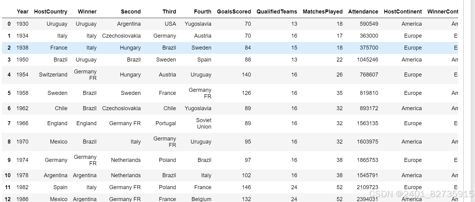 读取csv文件,该图为部分结果
# 查看数据表类型,进行必要的类型转化
hist_worldcup.dtypes

# 将字符串类型转化为整形
hist_worldcup['GoalsScored']= hist_worldcup["GoalsScored"].astype(int)
hist_worldcup['QualifiedTeams']= hist_worldcup["QualifiedTeams"].astype(int)
hist_worldcup['MatchesPlayed']= hist_worldcup["MatchesPlayed"].astype(int)
hist_worldcup['Attendance']= hist_worldcup["Attendance"].astype(int)
对数据类型进行转换
# 计算每届世界杯的平均进球数
hist_worldcup['AverageGoalsPerMatch'] = hist_worldcup['GoalsScored'] / hist_worldcup['MatchesPlayed']

# 绘制总参赛队伍数与平均进球数的散点图
plt.figure(figsize=(10, 6))
plt.scatter(hist_worldcup['MatchesPlayed'], hist_worldcup['AverageGoalsPerMatch'], color='blue')

# 设置标题字体大小
plt.title('平均进球数与总比赛场次的关系', fontsize=20)

# 设置x轴标签字体大小
plt.xlabel('总比赛场次数', fontsize=16)

# 设置y轴标签字体大小
plt.ylabel('平均进球数', fontsize=16)

# 设置网格
plt.grid(True)

# 显示图表
plt.show()

# 打印每届世界杯的平均进球数
print(hist_worldcup[['Year','MatchesPlayed','AverageGoalsPerMatch']])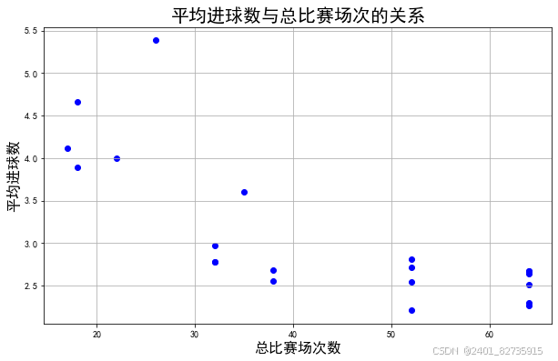
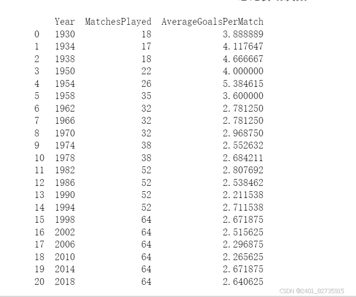 得到上图的结果
# 计算每届世界杯的平均进球数
hist_worldcup['AverageGoalsPerMatch'] = hist_worldcup['GoalsScored'] / hist_worldcup['MatchesPlayed']

# 绘制总参赛队伍数与平均进球数的散点图
plt.figure(figsize=(10, 6))
plt.scatter(hist_worldcup['QualifiedTeams'], hist_worldcup['AverageGoalsPerMatch'], color='green')

# 设置标题字体大小
plt.title('平均进球数与总参赛队伍数的关系', fontsize=20)

# 设置x轴标签字体大小
plt.xlabel('总参赛队伍数', fontsize=16)

# 设置y轴标签字体大小
plt.ylabel('平均进球数', fontsize=16)

# 设置网格
plt.grid(True)

# 设置x轴刻度为已有的总参赛队伍数
unique_teams = sorted(hist_worldcup['QualifiedTeams'].unique())
plt.xticks(unique_teams)

# 显示图表
plt.show()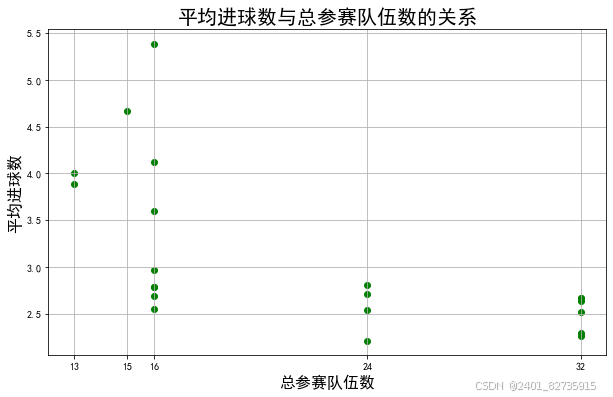
hist_worldcup['Decade'] = (hist_worldcup['Year'] // 10) * 10
grouped = hist_worldcup.groupby('Decade')
average_goals_per_decade = grouped['AverageGoalsPerMatch'].mean()
average_goals_per_decade
average_goals_per_decade.plot(kind='bar', color='skyblue')
plt.title('每个年代的世界杯平均进球数')
plt.xlabel('年代')
plt.ylabel('平均进球数')
plt.xticks(rotation=45)
plt.grid(axis='y')

# 显示图表
plt.show()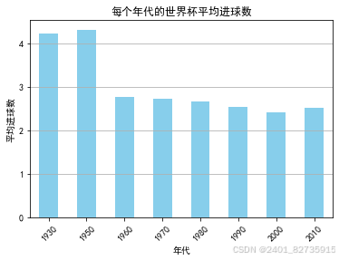
可以看出随着时代发展世界杯的场均进球数是呈下降趋势的,和印象中近几年越来越多的球队摆大巴踢防守反击不矛盾。
接下来我们预测2026年世界杯48支参赛队的场均进球数会发生什么变化。
hist_worldcup_1960_onward = hist_worldcup[hist_worldcup['Decade'] >= 1960]

# 使用线性回归模型进行拟合
X = hist_worldcup_1960_onward[['Decade']]
y = hist_worldcup_1960_onward['AverageGoalsPerMatch']

model = LinearRegression()
model.fit(X, y)

# 预测2020年代的平均进球数
predicted_goals_2020 = model.predict([[2020]])
predicted_goals_2020[0]
根据趋势预测2020年代的场均进球数,根据计算预测为一场比赛场均2.38个进球。
# 筛选出1960年代以后的数据
hist_worldcup_1960_onward = hist_worldcup[hist_worldcup['Year'] >= 1960]

# 确保数据类型正确
hist_worldcup_1960_onward['GoalsScored'] = hist_worldcup_1960_onward['GoalsScored'].astype(int)
hist_worldcup_1960_onward['QualifiedTeams'] = hist_worldcup_1960_onward['QualifiedTeams'].astype(int)
hist_worldcup_1960_onward['MatchesPlayed'] = hist_worldcup_1960_onward['MatchesPlayed'].astype(int)

# 计算平均进球数
hist_worldcup_1960_onward['AverageGoalsPerMatch'] = hist_worldcup_1960_onward['GoalsScored'] / hist_worldcup_1960_onward['MatchesPlayed']

# 定义自变量(特征)和因变量(目标变量)
X = hist_worldcup_1960_onward[['Year', 'QualifiedTeams', 'MatchesPlayed']]
y = hist_worldcup_1960_onward['AverageGoalsPerMatch']

# 创建线性回归模型
model = LinearRegression()

# 训练模型
model.fit(X, y)

# 输出模型参数
print('模型参数:', model.coef_)
print('截距:', model.intercept_)
这里进行计算线性回归模型的公式,算出最符合历史数据的参数。我们把这个模型归为理想化模型,即场均进球数只与历年来世界杯足球比赛风格的变化,参赛队伍数量的变化,以及比赛总场次的变化有关。通过观察表中数据和看球的认知,上世纪1960年代以前因为种种原因,比赛风格与后续差异较大。所以比赛风格因素我们只考虑1960年代以后。参赛队伍越多,参赛队伍的水平差距会变得更参差不齐。比赛场次的增加,会使球队变得更加疲惫,红黄牌导致球员停赛等等,降低预计场均进球数。

这是我们计算得到的参数
coefficients = np.array([-0.00020198, 0.0450475, -0.03234927])
intercept = 3.5510930569680035

# 2026年的数据
decade_2026 = 2026
qualified_teams_2026 = 48
matches_played_2026 = 104

# 使用多元线性回归模型计算2026年的平均进球数
average_goals_2026 = intercept + coefficients[0] * decade_2026 + coefficients[1] * qualified_teams_2026 + coefficients[2] * matches_played_2026
average_goals_2026
通过公式,我们计算2026届世界杯的预计场均进球数,计算的结果为1.94个场均进球。
接下来我们分析是否是东道主与比赛发挥的关系。
matches = pd.read_csv('WorldCupMatches.csv')读取csv文件,如果遇到编码问题请查阅相关资料改正。
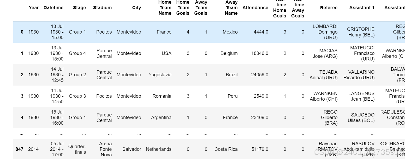 这是我们得到的部分结果。
# 类型转化
matches['Home Team Goals']= matches['Home Team Goals'].astype(int)
matches['Away Team Goals']= matches['Away Team Goals'].astype(int)

matches['result'] = matches['Home Team Goals'].astype(str)+"-"+matches['Away Team Goals'].astype(str)
matches
当然要进行类型转换。
def calculate_average_goals_per_match(year, host_countries, matches):
    # 筛选出该届世界杯的所有比赛
    world_cup_matches = matches[matches['Year'] == year]

    average_goals_per_host = {}
    for host_country in host_countries:
        individual_hosts = [host.strip() for host in host_country.split('/')]

        for individual_host in individual_hosts:
            # 找出东道主作为主队或客队的比赛
            host_matches1 = world_cup_matches[(world_cup_matches['Home Team Name'] == individual_host)]
            host_matches2 = world_cup_matches[(world_cup_matches['Away Team Name'] == individual_host)]
            # 统计东道主的进球总数
            total_goals = host_matches1['Home Team Goals'].sum() +host_matches2['Away Team Goals'].sum()

            # 计算东道主的比赛场数
            total_matches = len(host_matches1)+len(host_matches2)

            # 计算场均进球数
            average_goals = total_goals / total_matches if total_matches > 0 else 0

            average_goals_per_host[individual_host] = average_goals

    return average_goals_per_host

average_goals_per_world_cup = {}

# 分组以便处理每届世界杯
grouped_world_cups = hist_worldcup.groupby('Year')

# 遍历每一届世界杯
for year, group in grouped_world_cups:
    # 跳过2002届和1974届世界杯
    if year in [2002, 1974, 2018]:
        continue

    # 获取该届世界杯的东道主信息
    host_countries = group['HostCountry'].unique().tolist()
    # 使用辅助函数处理HostCountry值
    host_countries = [host for host in host_countries for single_host in host.split('/')]

    # 调用函数并存储结果
    average_goals_per_host = calculate_average_goals_per_match(year, host_countries, matches)
    average_goals_per_world_cup[year] = average_goals_per_host

for year, avg_goals in average_goals_per_world_cup.items():
    print(f"World Cup {year} - Hosts' Average Goals:")
    for host, avg in avg_goals.items():
        print(f"{host}: {avg:.2f} goals per match")
    print("\n")
我们自定义了一个函数,计算每届世界杯的东道主场均进球数。因为1974届,2002届世界杯的东道主特殊性,我们这里进行忽略处理。因为文件数据只有到2014届世界杯,所以后续2届世界杯我们也不予参考。最终我们得出了以下结果。
World Cup 1930 - Hosts' Average Goals:
Uruguay: 3.75 goals per match


World Cup 1934 - Hosts' Average Goals:
Italy: 2.40 goals per match


World Cup 1938 - Hosts' Average Goals:
France: 2.00 goals per match


World Cup 1950 - Hosts' Average Goals:
Brazil: 3.67 goals per match


World Cup 1954 - Hosts' Average Goals:
Switzerland: 2.75 goals per match


World Cup 1958 - Hosts' Average Goals:
Sweden: 2.00 goals per match


World Cup 1962 - Hosts' Average Goals:
Chile: 1.67 goals per match


World Cup 1966 - Hosts' Average Goals:
England: 1.83 goals per match


World Cup 1970 - Hosts' Average Goals:
Mexico: 1.50 goals per match


World Cup 1978 - Hosts' Average Goals:
Argentina: 2.14 goals per match


World Cup 1982 - Hosts' Average Goals:
Spain: 0.80 goals per match


World Cup 1986 - Hosts' Average Goals:
Mexico: 1.20 goals per match


World Cup 1990 - Hosts' Average Goals:
Italy: 1.43 goals per match


World Cup 1994 - Hosts' Average Goals:
USA: 0.75 goals per match


World Cup 1998 - Hosts' Average Goals:
France: 2.14 goals per match


World Cup 2006 - Hosts' Average Goals:
Germany: 2.00 goals per match


World Cup 2010 - Hosts' Average Goals:
South Africa: 1.00 goals per match


World Cup 2014 - Hosts' Average Goals:
Brazil: 1.36 goals per match
很明显每届世界杯的东道主表现都很突出呢
def calculate_average_goals_non_host(team, matches, host_years):
    # 筛选出球队参加的比赛
    team_matches1 = matches[(matches['Home Team Name'] == team)]
    team_matches2 = matches[(matches['Away Team Name'] == team)]
    # 筛选出球队作为东道主的年份
    host_years_team = host_years.get(team, [])
    # 筛选出球队非东道主参加的比赛
    non_host_matches1 = team_matches1[~team_matches1['Year'].isin(host_years_team)]
    non_host_matches2 = team_matches2[~team_matches2['Year'].isin(host_years_team)]
    # 统计球队在非东道主比赛中的进球总数
    total_goals = non_host_matches1['Home Team Goals'].sum() + non_host_matches2['Away Team Goals'].sum()

    # 计算球队在非东道主比赛中的比赛场数
    total_matches = len(non_host_matches1)+len(non_host_matches2)

    # 计算球队在非东道主比赛中的场均进球数
    average_goals = total_goals / total_matches if total_matches > 0 else 0

    return average_goals

# 创建一个字典来存储每届世界杯的东道主
host_years = {}
for year, hosts in average_goals_per_world_cup.items():
    for host in hosts.keys():
        if host not in host_years:
            host_years[host] = []
        host_years[host].append(year)

# 计算每个东道主在非东道主参加的世界杯比赛中的平均进球数
average_goals_non_host = {}
for host in host_years.keys():
    average_goals_non_host[host] = calculate_average_goals_non_host(host, matches, host_years)

# 打印结果
for team, avg in average_goals_non_host.items():
    print(f"{team}: {avg:.2f} goals per match in non-host World Cups")
再来计算这些国家在不是东道主的时候进行世界杯的场均进球数。
# 定义每张图中的国家数量
countries_per_plot = 3

# 创建一个空列表来存储每张图的索引
plot_indices = []

# 循环生成多张图片
for i in range(0, len(sorted_teams), countries_per_plot):
    # 获取当前图中的国家列表
    current_teams = sorted_teams[i:i+countries_per_plot]

    # 创建一个新的条形图
    fig, ax = plt.subplots()

    # 定义条形图的宽度
    bar_width = 0.35

    # 定义条形图的索引
    index = range(len(current_teams))

    # 创建两个条形图,分别代表东道主和非东道主的场均进球数
    bar1 = ax.bar(index, [combined_data[team][0] for team in current_teams], bar_width, label='东道主场均进球')
    bar2 = ax.bar([i + bar_width for i in index], [combined_data[team][1] for team in current_teams], bar_width, label='非东道主场均进球')

    # 添加标签和标题
    ax.set_xlabel('球队')
    ax.set_ylabel('场均进球')
    ax.set_title('部分国家在作为东道主和不是东道主的进球表现')
    ax.set_xticks([i + bar_width / 2 for i in index])
    ax.set_xticklabels(current_teams)
    ax.legend()

    # 保存当前图片的索引
    plot_indices.append(i)

    # 显示图片
    plt.tight_layout()
    plt.show()

plot_indices
为了方便看到数据的差异性。博主绘制了柱状图。
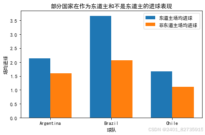
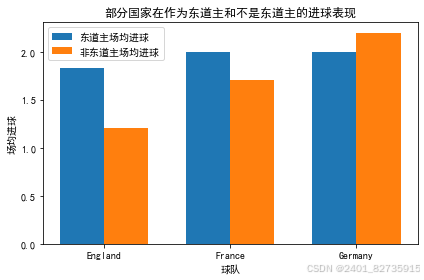
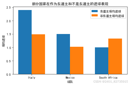
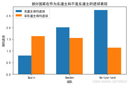
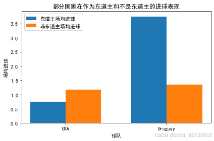
从结果可以看出,绝大部分东道主的表现还是有很大提升,也有几个国家在作为东道主的时候场均进球数有减少。
未完待续.......


 1万+
1万+

 被折叠的 条评论
为什么被折叠?
被折叠的 条评论
为什么被折叠?
 到【灌水乐园】发言


