2024年最新Python内存优化面试，深度学习进阶，多个输出和多个损失实现多标签分类，一线互联网大厂面试真题系统收录

2401_84121588

于 2024-04-23 11:15:23 发布

阅读量613

点赞数 5

分类专栏： 2024年程序员学习文章标签： python 面试深度学习

本文链接：https://blog.csdn.net/2401_84121588/article/details/138117379

版权

2024年程序员学习专栏收录该内容

12 篇文章 0 订阅

订阅专栏

收集整理了一份《2024年最新Python全套学习资料》免费送给大家，初衷也很简单，就是希望能够帮助到想自学提升又不知道该从何学起的朋友。

既有适合小白学习的零基础资料，也有适合3年以上经验的小伙伴深入学习提升的进阶课程，涵盖了95%以上Python知识点，真正体系化！

由于文件比较多，这里只是将部分目录截图出来

如果你需要这些资料，可以添加V无偿获取：hxbc188 （备注666）

正文

@staticmethod

def build(width, height, numCategories, numColors,

finalAct=“softmax”):

initialize the input shape and channel dimension (this code

assumes you are using TensorFlow which utilizes channels

last ordering)

inputShape = (height, width, 3)

chanDim = -1

construct both the “category” and “color” sub-networks

inputs = Input(shape=inputShape)

categoryBranch = FashionNet.build_category_branch(inputs,

numCategories, finalAct=finalAct, chanDim=chanDim)

colorBranch = FashionNet.build_color_branch(inputs,

numColors, finalAct=finalAct, chanDim=chanDim)

create the model using our input (the batch of images) and

two separate outputs – one for the clothing category

branch and another for the color branch, respectively

model = Model(

inputs=inputs,

outputs=[categoryBranch, colorBranch],

name=“fashionnet”)

return the constructed network architecture

return model

定义build函数，有5个参数。 build 函数假设我们使用的是 TensorFlow 和最后一次排序的通道。

inputShape 元组是明确排序的 (height, width, 3) ，其中 3 代表 RGB 通道。如果您想使用 TensorFlow 以外的后端，您需要修改代码以：(1) 正确地为您的后端设置正确的通道顺序，以及 (2) 实现一个自定义层来处理 RGB 到灰度的转换。从那里，我们定义了网络的两个分支，然后将它们放在一个模型中。关键是我们的分支有一个共同的输入，但有两个不同的输出（服装类型和颜色分类）。

实现多输出和多损失训练脚本

========================================================================

现在我们已经实现了我们的 FashionNet 架构，让我们训练它！准备好后，打开 train.py 并深入研究：

set the matplotlib backend so figures can be saved in the background

import matplotlib

matplotlib.use(“Agg”)

import the necessary packages

from tensorflow.keras.optimizers import Adam

from tensorflow.keras.preprocessing.image import img_to_array

from sklearn.preprocessing import LabelBinarizer

from sklearn.model_selection import train_test_split

from model.fashionnet import FashionNet

from imutils import paths

import matplotlib.pyplot as plt

import numpy as np

import argparse

import random

import pickle

import cv2

import os

我们首先为脚本导入必要的包。

从那里我们解析我们的命令行参数：

construct the argument parser and parse the arguments

ap = argparse.ArgumentParser()

ap.add_argument(“-d”, “–dataset”, required=True,

help=“path to input dataset (i.e., directory of images)”)

ap.add_argument(“-m”, “–model”, required=True,

help=“path to output model”)

ap.add_argument(“-l”, “–categorybin”, required=True,

help=“path to output category label binarizer”)

ap.add_argument(“-c”, “–colorbin”, required=True,

help=“path to output color label binarizer”)

ap.add_argument(“-p”, “–plot”, type=str, default=“output”,

help=“base filename for generated plots”)

args = vars(ap.parse_args())

我们很快就会看到如何运行训练脚本。现在，只知道 --dataset 是我们数据集的输入文件路径， --model 、 --categorybin 、 --colorbin 都是三个输出文件路径。

或者，您可以使用 --plot 参数为生成的精度/损失图指定基本文件名。

现在，让我们建立四个重要的训练变量：

initialize the number of epochs to train for, initial learning rate,

batch size, and image dimensions

EPOCHS = 50

INIT_LR = 1e-3

BS = 32

IMAGE_DIMS = (96, 96, 3)

我们设置以下变量：

EPOCHS : epoch 数设置为 50 。通过实验，我发现 50 个 epoch 生成的模型具有低损失并且没有过拟合到训练集（或尽可能不过拟合）。
INIT_LR ：我们的初始学习率设置为 0.001 。学习率控制着我们沿着梯度所做的“步骤”。较小的值表示较小的步长，较大的值表示较大的步长。我们很快就会看到我们将使用 Adam 优化器，同时随着时间的推移逐渐降低学习率。
BS：我们将以 32 的批量大小训练我们的网络。
IMAGE_DIMS ：所有输入图像都将调整为 96 x 96，具有 3 个通道 (RGB)。我们正在使用这些维度进行训练，我们的网络架构输入维度也反映了这些维度。当我们在后面的部分中使用示例图像测试我们的网络时，测试维度必须与训练维度匹配。

我们的下一步是抓取我们的图像路径并随机打乱它们。我们还将初始化列表以分别保存图像本身以及服装类别和颜色：

grab the image paths and randomly shuffle them

print(“[INFO] loading images…”)

imagePaths = sorted(list(paths.list_images(args[“dataset”])))

random.seed(42)

random.shuffle(imagePaths)

initialize the data, clothing category labels (i.e., shirts, jeans,

dresses, etc.) along with the color labels (i.e., red, blue, etc.)

data = []

categoryLabels = []

colorLabels = []

随后，我们将遍历 imagePaths 、预处理并填充 data 、 categoryLabels 和 colorLabels 列表：

loop over the input images

for imagePath in imagePaths:

load the image, pre-process it, and store it in the data list

image = cv2.imread(imagePath)

image = cv2.resize(image, (IMAGE_DIMS[1], IMAGE_DIMS[0]))

image = cv2.cvtColor(image, cv2.COLOR_BGR2RGB)

image = img_to_array(image)

data.append(image)

extract the clothing color and category from the path and

update the respective lists

(color, cat) = imagePath.split(os.path.sep)[-2].split(“_”)

categoryLabels.append(cat)

colorLabels.append(color)

我们开始遍历我们的 imagePaths。

在循环内部，我们加载图像并将其调整为 IMAGE_DIMS 。我们还将图像从 BGR 排序转换为 RGB。我们为什么要进行这种转换？回想一下我们在 build_category_branch 函数中的 FashionNet 类，我们在 Lambda 函数/层中使用了 TensorFlow 的 rgb_to_grayscale 转换。因此，我们首先转换为 RGB，并最终将预处理后的图像附加到数据列表中。

接下来，仍然在循环内部，我们从当前图像所在的目录名称中提取颜色和类别标签。

要查看此操作，只需在终端中启动 Python，并提供一个示例 imagePath 进行实验，如下所示：

$ python

import os

imagePath = “dataset/red_dress/00000000.jpg”

(color, cat) = imagePath.split(os.path.sep)[-2].split(“_”)

color

‘red’

cat

‘dress’

您当然可以按您希望的任何方式组织您的目录结构（但您必须修改代码）。我最喜欢的两种方法包括 (1) 为每个标签使用子目录或 (2) 将所有图像存储在单个目录中，然后创建 CSV 或 JSON 文件以将图像文件名映射到它们的标签。让我们将三个列表转换为 NumPy 数组，对标签进行二值化，并将数据划分为训练和测试分割：

scale the raw pixel intensities to the range [0, 1] and convert to

a NumPy array

data = np.array(data, dtype=“float”) / 255.0

print(“[INFO] data matrix: {} images ({:.2f}MB)”.format(

len(imagePaths), data.nbytes / (1024 * 1000.0)))

convert the label lists to NumPy arrays prior to binarization

categoryLabels = np.array(categoryLabels)

colorLabels = np.array(colorLabels)

binarize both sets of labels

print(“[INFO] binarizing labels…”)

categoryLB = LabelBinarizer()

colorLB = LabelBinarizer()

categoryLabels = categoryLB.fit_transform(categoryLabels)

colorLabels = colorLB.fit_transform(colorLabels)

partition the data into training and testing splits using 80% of

the data for training and the remaining 20% for testing

split = train_test_split(data, categoryLabels, colorLabels,

test_size=0.2, random_state=42)

(trainX, testX, trainCategoryY, testCategoryY,

trainColorY, testColorY) = split

我们的最后一个预处理步骤——转换为 NumPy 数组并将原始像素强度缩放为 [0, 1]。

我们还将 categoryLabels 和 colorLabels 转换为 NumPy 数组。这是必要的，因为在我们的下一个中，我们将使用我们之前导入的 scikit-learn 的 LabelBinarizer对标签进行二值化。由于我们的网络有两个独立的分支，我们可以使用两个独立的标签二值化器——这与我们使用 MultiLabelBinarizer（也来自 scikit-learn）的多标签分类不同。

接下来，我们对数据集执行典型的 80% 训练/20% 测试拆分。

让我们构建网络，定义我们的独立损失，并编译我们的模型：

initialize our FashionNet multi-output network

model = FashionNet.build(96, 96,

numCategories=len(categoryLB.classes_),

numColors=len(colorLB.classes_),

finalAct=“softmax”)

define two dictionaries: one that specifies the loss method for

each output of the network along with a second dictionary that

specifies the weight per loss

losses = {

“category_output”: “categorical_crossentropy”,

“color_output”: “categorical_crossentropy”,

}

lossWeights = {“category_output”: 1.0, “color_output”: 1.0}

initialize the optimizer and compile the model

print(“[INFO] compiling model…”)

opt = Adam(lr=INIT_LR, decay=INIT_LR / EPOCHS)

model.compile(optimizer=opt, loss=losses, loss_weights=lossWeights,

metrics=[“accuracy”])

实例化多输出 FashionNet 模型。我们在创建 FashionNet 类并在其中构建函数时剖析了参数，因此请务必查看我们在此处实际提供的值。

接下来，我们需要为每个完全连接的头部定义两个损失。

定义多个损失是通过使用每个分支激活层的名称的字典来完成的——这就是我们在 FashionNet 实现中命名输出层的原因！每个损失都将使用分类交叉熵，这是训练网络进行大于 2 类分类时使用的标准损失方法。

我们还在单独字典（具有相同值的同名键）中定义了相等的 lossWeights。在您的特定应用程序中，您可能希望对一个损失进行比另一个更重的加权。

现在我们已经实例化了我们的模型并创建了 loss + lossWeights 字典，让我们用学习率衰减初始化 Adam 优化器并编译我们的模型。

我们的下一个块只是开始训练过程：

train the network to perform multi-output classification

H = model.fit(x=trainX,

y={“category_output”: trainCategoryY, “color_output”: trainColorY},

validation_data=(testX,

{“category_output”: testCategoryY, “color_output”: testColorY}),

epochs=EPOCHS,

verbose=1)

save the model to disk

print(“[INFO] serializing network…”)

model.save(args[“model”], save_format=“h5”)

请注意，对于 TensorFlow 2.0+，我们建议明确设置 save_format=“h5”（HDF5 格式）。

回想一下第 87-90 行，我们将数据拆分为训练 (trainX) 和测试 (testX)。在第 114-119 行，我们在提供数据的同时启动了训练过程。请注意第 115 行，我们将标签作为字典传入。第 116 行和第 117 行也是如此，我们为验证数据传入了一个 2 元组。在使用 Keras 执行多输出分类时，需要以这种方式传递训练和验证标签。我们需要指示 Keras 哪一组目标标签对应于网络的哪个输出分支。使用我们的命令行参数 (args[“model”] )，我们将序列化模型保存到磁盘以备将来调用。我们也会做同样的事情来将我们的标签二值化器保存为序列化的 pickle 文件：

save the category binarizer to disk

print(“[INFO] serializing category label binarizer…”)

f = open(args[“categorybin”], “wb”)

f.write(pickle.dumps(categoryLB))

f.close()

save the color binarizer to disk

print(“[INFO] serializing color label binarizer…”)

f = open(args[“colorbin”], “wb”)

f.write(pickle.dumps(colorLB))

f.close()

使用命令行参数路径（args[“categorybin”] 和 args[“colorbin”]），我们将两个标签二值化器（categoryLB 和 colorLB）写入磁盘上的序列化 pickle 文件。

从那里开始，就是在这个脚本中绘制结果：

plot the total loss, category loss, and color loss

lossNames = [“loss”, “category_output_loss”, “color_output_loss”]

plt.style.use(“ggplot”)

(fig, ax) = plt.subplots(3, 1, figsize=(13, 13))

loop over the loss names

for (i, l) in enumerate(lossNames):

plot the loss for both the training and validation data

title = “Loss for {}”.format(l) if l != “loss” else “Total loss”

ax[i].set_title(title)

ax[i].set_xlabel(“Epoch #”)

ax[i].set_ylabel(“Loss”)

ax[i].plot(np.arange(0, EPOCHS), H.history[l], label=l)

ax[i].plot(np.arange(0, EPOCHS), H.history[“val_” + l],

label=“val_” + l)

ax[i].legend()

save the losses figure

plt.tight_layout()

plt.savefig(“{}_losses.png”.format(args[“plot”]))

plt.close()

上面的代码块负责在单独但堆叠的图上绘制每个损失函数的损失历史，包括：

总体损耗
类别输出的损失
颜色输出的损失

同样，我们将在单独的图像文件中绘制精度：

create a new figure for the accuracies

accuracyNames = [“category_output_accuracy”, “color_output_accuracy”]

plt.style.use(“ggplot”)

(fig, ax) = plt.subplots(2, 1, figsize=(8, 8))

loop over the accuracy names

for (i, l) in enumerate(accuracyNames):

plot the loss for both the training and validation data

ax[i].set_title(“Accuracy for {}”.format(l))

ax[i].set_xlabel(“Epoch #”)

ax[i].set_ylabel(“Accuracy”)

ax[i].plot(np.arange(0, EPOCHS), H.history[l], label=l)

ax[i].plot(np.arange(0, EPOCHS), H.history[“val_” + l],

label=“val_” + l)

ax[i].legend()

save the accuracies figure

plt.tight_layout()

plt.savefig(“{}_accs.png”.format(args[“plot”]))

plt.close()

训练多输出/多损失 Keras 模型

=============================================================================

打开终端。然后粘贴以下命令以开始训练过程：

$ python train.py --dataset dataset --model output/fashion.model \

–categorybin output/category_lb.pickle --colorbin output/color_lb.pickle

Using TensorFlow backend.

[INFO] loading images…

[INFO] data matrix: 2521 images (544.54MB)

[INFO] loading images…

[INFO] data matrix: 2521 images (544.54MB)

[INFO] binarizing labels…

[INFO] compiling model…

Epoch 1/50

63/63 [==============================] - 1s 20ms/step - loss: 0.8523 - category_output_loss: 0.5301 - color_output_loss: 0.3222 - category_output_accuracy: 0.8264 - color_output_accuracy: 0.8780 - val_loss: 3.6909 - val_category_output_loss: 1.8052 - val_color_output_loss: 1.8857 - val_category_output_accuracy: 0.3188 - val_color_output_accuracy: 0.4416

Epoch 2/50

63/63 [==============================] - 1s 14ms/step - loss: 0.4367 - category_output_loss: 0.3092 - color_output_loss: 0.1276 - category_output_accuracy: 0.9033 - color_output_accuracy: 0.9519 - val_loss: 7.0533 - val_category_output_loss: 2.9279 - val_color_output_loss: 4.1254 - val_category_output_accuracy: 0.3188 - val_color_output_accuracy: 0.4416

Epoch 3/50

63/63 [==============================] - 1s 14ms/step - loss: 0.2892 - category_output_loss: 0.1952 - color_output_loss: 0.0940 - category_output_accuracy: 0.9350 - color_output_accuracy: 0.9653 - val_loss: 6.2512 - val_category_output_loss: 2.0540 - val_color_output_loss: 4.1972 - val_category_output_accuracy: 0.4020 - val_color_output_accuracy: 0.4416

…

Epoch 48/50

63/63 [==============================] - 1s 14ms/step - loss: 0.0189 - category_output_loss: 0.0106 - color_output_loss: 0.0083 - category_output_accuracy: 0.9960 - color_output_accuracy: 0.9970 - val_loss: 0.2625 - val_category_output_loss: 0.2250 - val_color_output_loss: 0.0376 - val_category_output_accuracy: 0.9564 - val_color_output_accuracy: 0.9861

Epoch 49/50

63/63 [==============================] - 1s 14ms/step - loss: 0.0190 - category_output_loss: 0.0041 - color_output_loss: 0.0148 - category_output_accuracy: 0.9985 - color_output_accuracy: 0.9950 - val_loss: 0.2333 - val_category_output_loss: 0.1927 - val_color_output_loss: 0.0406 - val_category_output_accuracy: 0.9604 - val_color_output_accuracy: 0.9881

Epoch 50/50

63/63 [==============================] - 1s 14ms/step - loss: 0.0188 - category_output_loss: 0.0046 - color_output_loss: 0.0142 - category_output_accuracy: 0.9990 - color_output_accuracy: 0.9960 - val_loss: 0.2140 - val_category_output_loss: 0.1719 - val_color_output_loss: 0.0421 - val_category_output_accuracy: 0.9624 - val_color_output_accuracy: 0.9861

[INFO] serializing network…

[INFO] serializing category label binarizer…

[INFO] serializing color label binarizer…

对于我们的类别输出，我们获得了：

训练集上 99.90% 的准确率
在测试集上的准确率为 96.24%

对于我们达到的颜色输出：

99.60% 的训练集准确率
在测试集上的准确率为 98.61%

您可以在下面找到我们多个损失中的每一个的图：

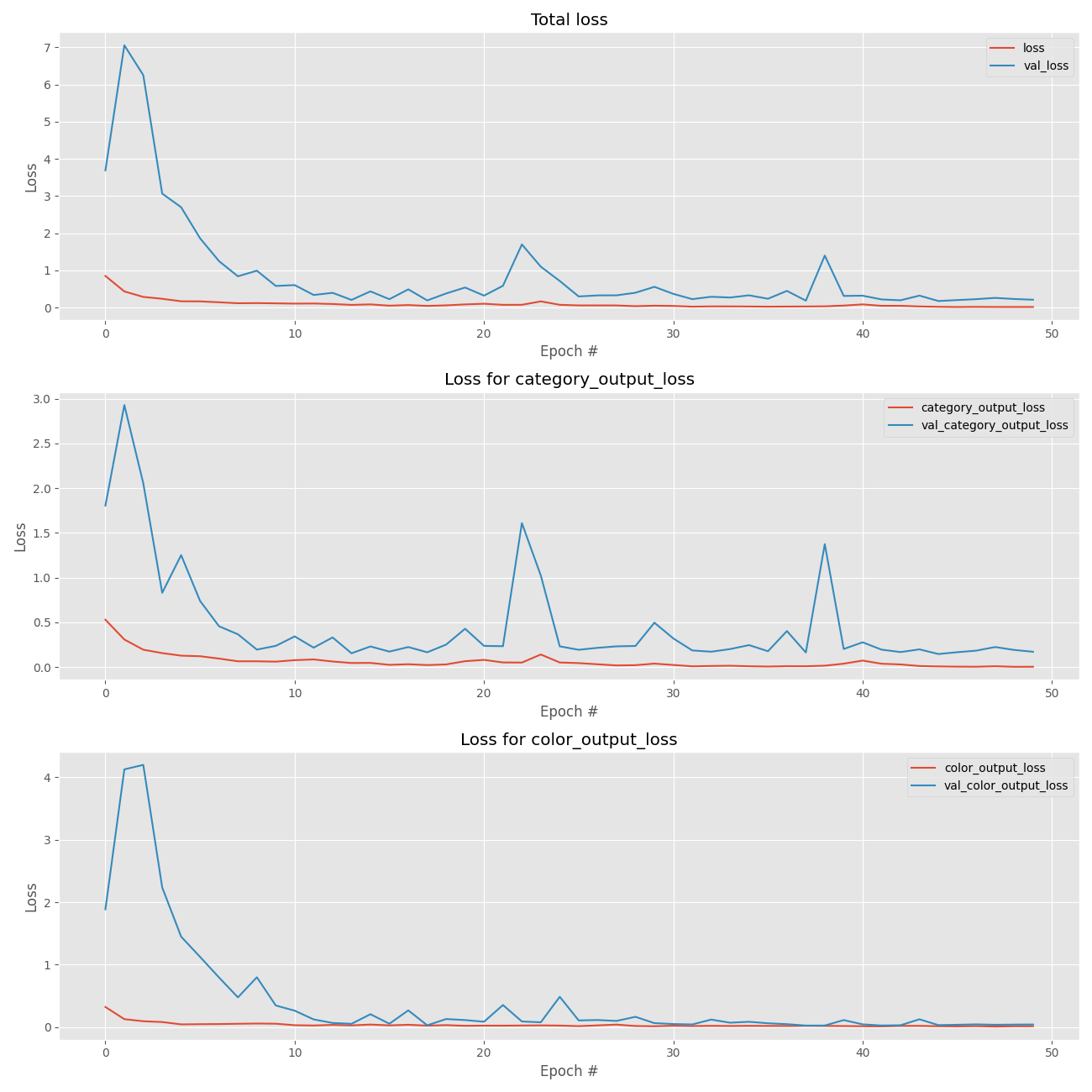
图 7：我们的 Keras 深度学习多输出分类训练损失是用 matplotlib 绘制的。我们的总损失（顶部）、服装类别损失（中间）和颜色损失（底部）被独立绘制以供分析。

以及我们的多重精度：

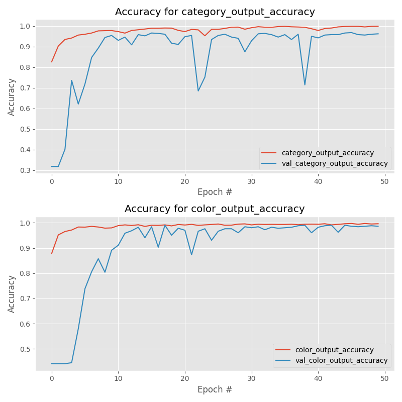
图 8：FashionNet，一个多输出分类网络，用 Keras 训练。为了分析训练，最好在单独的图中显示准确度。服装类别训练准确率图（上）。颜色训练精度图（底部）。

实现多输出分类脚本

====================================================================

打开classify.py，插入如下代码：

import the necessary packages

from tensorflow.keras.preprocessing.image import img_to_array

from tensorflow.keras.models import load_model

import tensorflow as tf

import numpy as np

import argparse

import imutils

import pickle

import cv2

construct the argument parser and parse the arguments

ap = argparse.ArgumentParser()

ap.add_argument(“-m”, “–model”, required=True,

help=“path to trained model model”)

ap.add_argument(“-l”, “–categorybin”, required=True,

help=“path to output category label binarizer”)

ap.add_argument(“-c”, “–colorbin”, required=True,

help=“path to output color label binarizer”)

ap.add_argument(“-i”, “–image”, required=True,

help=“path to input image”)

args = vars(ap.parse_args())

我们有四个命令行参数，这些参数是在您的终端中运行此脚本所必需的：

–model ：我们刚刚训练的序列化模型文件的路径（我们之前脚本的输出）。
–categorybin ：类别标签二值化器的路径（我们之前脚本的输出）。
–colorbin ：颜色标签二值化器的路径（我们之前脚本的输出）。
–image ：我们的测试图像文件路径——这个图像将来自我们的 examples/ 目录。

从那里，我们加载我们的图像并对其进行预处理：

load the image

image = cv2.imread(args[“image”])

output = imutils.resize(image, width=400)

image = cv2.cvtColor(image, cv2.COLOR_BGR2RGB)

pre-process the image for classification

image = cv2.resize(image, (96, 96))

image = image.astype(“float”) / 255.0

image = img_to_array(image)

image = np.expand_dims(image, axis=0)

在我们运行推理之前需要预处理我们的图像。在上面的块中，我们加载图像，调整其大小以用于输出目的，并交换颜色通道，以便我们可以在 FashionNet 的 Lambda 层中使用 TensorFlow 的 RGB 灰度函数。然后我们调整 RGB 图像的大小（从我们的训练脚本中调用 IMAGE_DIMS），将其缩放为 [0, 1]，转换为 NumPy 数组，并为批次添加维度。

预处理步骤遵循在我们的训练脚本中采取的相同操作是至关重要的。

接下来，让我们加载我们的序列化模型和两个标签二值化器：

load the trained convolutional neural network from disk, followed

by the category and color label binarizers, respectively

print(“[INFO] loading network…”)

model = load_model(args[“model”], custom_objects={“tf”: tf})

categoryLB = pickle.loads(open(args[“categorybin”], “rb”).read())

colorLB = pickle.loads(open(args[“colorbin”], “rb”).read())

使用四个命令行参数中的三个，我们加载 model 、 categoryLB 和 colorLB 。

现在多输出 Keras 模型和标签二值化器都在内存中，我们可以对图像进行分类：

classify the input image using Keras’ multi-output functionality

print(“[INFO] classifying image…”)

(categoryProba, colorProba) = model.predict(image)

find indexes of both the category and color outputs with the

largest probabilities, then determine the corresponding class

labels

categoryIdx = categoryProba[0].argmax()

colorIdx = colorProba[0].argmax()

categoryLabel = categoryLB.classes_[categoryIdx]

colorLabel = colorLB.classes_[colorIdx]

执行多输出分类，得出类别和颜色的概率（分别为 categoryProba 和 colorProba）。

注意：我没有包含包含代码，因为它有点冗长，但您可以通过检查输出张量的名称来确定 TensorFlow + Keras 模型返回多个输出的顺序。

从那里，我们将提取类别和颜色的最高概率指数。使用高概率指数，我们可以提取类名。这似乎有点太容易了，不是吗？但这就是使用 Keras 将多输出分类应用于新输入图像的全部内容！

让我们显示结果来证明它：

draw the category label and color label on the image

categoryText = “category: {} ({:.2f}%)”.format(categoryLabel,

categoryProba[0][categoryIdx] * 100)

colorText = “color: {} ({:.2f}%)”.format(colorLabel,

colorProba[0][colorIdx] * 100)

cv2.putText(output, categoryText, (10, 25), cv2.FONT_HERSHEY_SIMPLEX,

0.7, (0, 255, 0), 2)

cv2.putText(output, colorText, (10, 55), cv2.FONT_HERSHEY_SIMPLEX,

0.7, (0, 255, 0), 2)

display the predictions to the terminal as well

print(“[INFO] {}”.format(categoryText))

print(“[INFO] {}”.format(colorText))

show the output image

cv2.imshow(“Output”, output)

cv2.waitKey(0)

我们在输出图像上显示结果。如果我们遇到“红色连衣裙”，它会在左上角的绿色文本中看起来像这样：类别：连衣裙 (89.04%) 颜色：红色（95.07%）相同的信息打印到终端，之后输出图像显示在屏幕上。

使用 Keras 执行多输出分类

===========================================================================

最后

Python崛起并且风靡，因为优点多、应用领域广、被大牛们认可。学习 Python 门槛很低，但它的晋级路线很多，通过它你能进入机器学习、数据挖掘、大数据，CS等更加高级的领域。Python可以做网络应用，可以做科学计算，数据分析，可以做网络爬虫，可以做机器学习、自然语言处理、可以写游戏、可以做桌面应用…Python可以做的很多，你需要学好基础，再选择明确的方向。这里给大家分享一份全套的 Python 学习资料，给那些想学习 Python 的小伙伴们一点帮助！

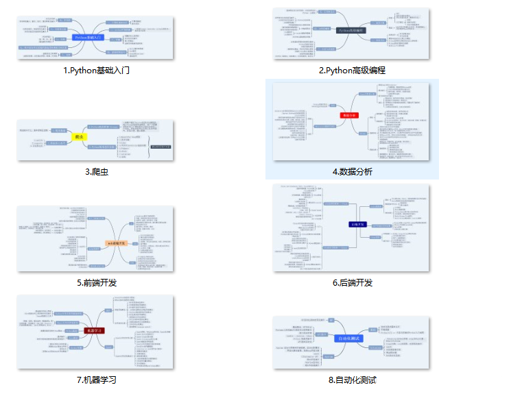
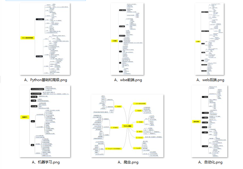
👉Python所有方向的学习路线👈

Python所有方向的技术点做的整理，形成各个领域的知识点汇总，它的用处就在于，你可以按照上面的知识点去找对应的学习资源，保证自己学得较为全面。

👉Python必备开发工具👈

工欲善其事必先利其器。学习Python常用的开发软件都在这里了，给大家节省了很多时间。

👉Python全套学习视频👈

我们在看视频学习的时候，不能光动眼动脑不动手，比较科学的学习方法是在理解之后运用它们，这时候练手项目就很适合了。

👉实战案例👈

学python就与学数学一样，是不能只看书不做题的，直接看步骤和答案会让人误以为自己全都掌握了，但是碰到生题的时候还是会一筹莫展。

因此在学习python的过程中一定要记得多动手写代码，教程只需要看一两遍即可。

👉大厂面试真题👈

我们学习Python必然是为了找到高薪的工作，下面这些面试题是来自阿里、腾讯、字节等一线互联网大厂最新的面试资料，并且有阿里大佬给出了权威的解答，刷完这一套面试资料相信大家都能找到满意的工作。