深度学习入门，Keras Conv2D类参数详解

图9: Keras 为 Conv2D 类提供了许多初始化器。 初始化器可用于帮助更有效地训练更深的神经网络。

kernel_initializer 控制用于在实际训练网络之前初始化 Conv2D 类中的所有值的初始化方法。 类似地，bias_initializer 控制在训练开始之前如何初始化偏置向量。 完整的初始化器列表可以在 Keras 文档中找到； 但是，这是我的建议：

1、不理会bias_initialization——默认情况下它会用零填充（你很少，如果有的话，必须改变bias初始化方法）。

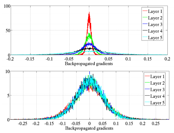
2、kernel_initializer 默认为 glorot_uniform ，这是 Xavier Glorot 统一初始化方法，对于大多数任务来说是完美的； 然而，对于更深层的神经网络，您可能希望使用 he_normal（MSRA/He 等人的初始化），当您的网络具有大量参数（即 VGGNet）时，该方法特别有效。

在我实现的绝大多数 CNN 中，我要么使用 glorot_uniform 要么使用 he_normal——我建议你也这样做，除非你有特定的理由使用不同的初始化程序。

kernel_regularizer、bias_regularizer 和 activity_regularizer

========================================================================================================================

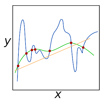
图10: 应该调整正则化超参数，尤其是在处理大型数据集和非常深的网络时。 我经常调整 kernel_regularizer 参数以减少过度拟合并增加模型泛化到不熟悉的图像的能力。

kernel_regularizer 、bias_regularizer 和 activity_regularizer 控制应用于 Conv2D 层的正则化方法的类型和数量。 应用正则化可以帮助您： 减少过拟合的影响 提高模型的泛化能力 在处理大型数据集和深度神经网络时，应用正则化通常是必须的。 通常你会遇到应用 L1 或 L2 正则化的情况——如果我检测到过度拟合的迹象，我将在我的网络上使用 L2 正则化：

from tensorflow.keras.regularizers import l2

…

model.add(Conv2D(32, (3, 3), activation=“relu”),

kernel_regularizer=l2(0.0005))

您应用的正则化量是您需要针对自己的数据集进行调整的超参数，但我发现 0.0001-0.001 的值是一个很好的开始范围。

我建议不要管你的偏差正则化器——正则化偏差通常对减少过度拟合的影响很小。

我还建议将 activity_regularizer 保留为其默认值（即，没有活动正则化）。

虽然权重正则化方法对权重本身进行操作，f(W)，其中 f 是激活函数，W 是权重，但活动正则化器对输出 f(O) 进行操作，其中 O 是层的输出。

除非有非常具体的原因，您希望对输出进行正则化，否则最好不要理会这个参数。

kernel_constraint 和bias_constraint

===============================================================================================

Keras Conv2D 类的最后两个参数是 kernel_constraint 和 bias_constraint 。

这些参数允许您对 Conv2D 层施加约束，包括非负性、单位归一化和最小-最大归一化。

您可以在 Keras 文档中查看受支持约束的完整列表。

同样，除非您有特定原因对 Conv2D 层施加约束，否则我建议您单独保留内核约束和偏差约束。

CALTECH-101（子集）数据集

=============================================================================

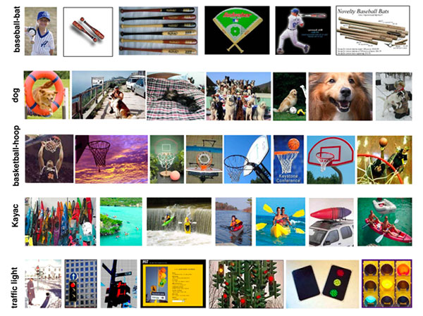
图11: CALTECH-101 数据集包含 101 个对象类别，每个类别有 40-80 张图像。 今天博客文章示例的数据集仅包含其中 4 个类：人脸、豹子、摩托车和飞机（来源）。

CALTECH-101 数据集是一个包含 101 个对象类别的数据集，每个类别有 40 到 800 张图像。

大多数图像每类大约有 50 张图像。

数据集的目标是训练一个能够预测目标类别的模型。 在神经网络和深度学习重新兴起之前，最先进的准确率仅为约 65%。

然而，通过使用卷积神经网络，可以达到 90% 以上的准确率（正如 He 等人在他们 2014 年的论文《用于视觉识别的深度卷积网络中的空间金字塔池化》中所证明的那样）。

今天，我们将在数据集的 4 类子集上实现一个简单而有效的 CNN，它能够达到 96% 以上的准确率：

• Faces: 436 images

• Leopards: 201 images

• Motorbikes: 799 images

• Airplanes: 801 images

我们使用数据集的子集的原因是，即使您没有 GPU，您也可以轻松地按照此示例从头开始训练网络。

同样，本教程的目的并不是要在 CALTECH-101 上提供最先进的结果——而是要教您如何使用 Keras 的 Conv2D 类来实现和训练自定义卷积神经网络的基础知识 .

项目结构

===============================================================

数据集地址：

http://www.vision.caltech.edu/Image_Datasets/Caltech101/101_ObjectCategories.tar.gz

linux下载指令：

$ wget http://www.vision.caltech.edu/Image_Datasets/Caltech101/101_ObjectCategories.tar.gz

$ tar -zxvf 101_ObjectCategories.tar.gz

项目的树结构

$ tree --dirsfirst -L 2 -v

.

├── 101_ObjectCategories

…

│ ├── Faces [436 entries]

…

│ ├── Leopards [201 entries]

│ ├── Motorbikes [799 entries]

…

│ ├── airplanes [801 entries]

…

├── pyimagesearch

│ ├── init.py

│ └── stridednet.py

├── 101_ObjectCategories.tar.gz

├── train.py

└── plot.png

第一个目录 101_ObjectCategories/ 是我们在上一节中提取的数据集。 它包含 102 个文件夹，因此我删除了今天的博客文章我们不关心的行。 剩下的是前面讨论过的四个对象类别的子集。

pyimagesearch/ 模块不可通过 pip 安装。 您必须使用“下载”来获取文件。 在该模块中，您将找到包含 StrdedNet 类的 stridendet.py。

除了 stridednet.py 之外，我们还将查看根文件夹中的 train.py。 我们的训练脚本将使用 StridedNet 和我们的小数据集来训练模型以用于示例目的。

训练脚本将生成训练历史图 plot.png 。

Keras Conv2D 示例

==========================================================================

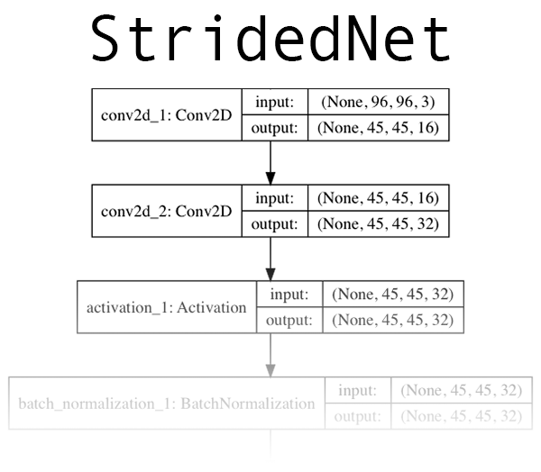
图12: 一个名为“StridedNet”的深度学习 CNN 作为今天关于 Keras Conv2D 参数的博客文章的示例。 点击 展开。

现在我们已经回顾了 (1) Keras Conv2D 类的工作原理和 (2) 我们将训练网络的数据集，让我们继续实施我们将训练的卷积神经网络。 我们今天将使用的 CNN，“StridedNet”，是我为本教程的目的而编写的。 StridedNet 具有三个重要的特性：

它使用跨步卷积而不是池化操作来减小体积大小

第一个 CONV 层使用 7×7 过滤器，但网络中的所有其他层使用 3×3 过滤器（类似于 VGG）

MSRA/He 等人。 正态分布算法用于初始化网络中的所有权重

现在让我们继续并实施 StridedNet。

打开一个新文件，将其命名为 stridednet.py ，并插入以下代码：

import the necessary packages

from tensorflow.keras.models import Sequential

from tensorflow.keras.layers import BatchNormalization

from tensorflow.keras.layers import Conv2D

from tensorflow.keras.layers import Activation

from tensorflow.keras.layers import Flatten

from tensorflow.keras.layers import Dropout

from tensorflow.keras.layers import Dense

from tensorflow.keras import backend as K

class StridedNet:

@staticmethod

def build(width, height, depth, classes, reg, init=“he_normal”):

initialize the model along with the input shape to be

“channels last” and the channels dimension itself

model = Sequential()

inputShape = (height, width, depth)

chanDim = -1

if we are using “channels first”, update the input shape

and channels dimension

if K.image_data_format() == “channels_first”:

inputShape = (depth, height, width)

chanDim = 1

我们所有的 Keras 模块都在第 2-9 行导入，即 Conv2D。

我们的 StrdedNet 类在第 11 行定义，在第 13 行使用单个构建方法。

build 方法接受六个参数：

​ width ：图像宽度（以像素为单位）。

​ height ：以像素为单位的图像高度。

​ depth ：图像的通道数。

​ classes ：模型需要预测的类数。

​ reg : 正则化方法。

​ init ：内核初始化程序。

​ width 、 height 和 depth 参数影响输入体积形状。

对于“channels_last”排序，输入形状在第 17 行指定，其中深度是最后一个。 我们可以使用 Keras 后端检查 image_data_format 以查看我们是否需要适应“channels_first”排序（第 22-24 行）。 让我们看看如何构建前三个 CONV 层：

our first CONV layer will learn a total of 16 filters, each

Of which are 7x7 – we’ll then apply 2x2 strides to reduce

the spatial dimensions of the volume

model.add(Conv2D(16, (7, 7), strides=(2, 2), padding=“valid”,

kernel_initializer=init, kernel_regularizer=reg,

input_shape=inputShape))

here we stack two CONV layers on top of each other where

each layerswill learn a total of 32 (3x3) filters

model.add(Conv2D(32, (3, 3), padding=“same”,

kernel_initializer=init, kernel_regularizer=reg))

model.add(Activation(“relu”))

model.add(BatchNormalization(axis=chanDim))

model.add(Conv2D(32, (3, 3), strides=(2, 2), padding=“same”,

kernel_initializer=init, kernel_regularizer=reg))

model.add(Activation(“relu”))

model.add(BatchNormalization(axis=chanDim))

model.add(Dropout(0.25))

每个 Conv2D 都使用 model.add 堆叠在网络上。

请注意，对于第一个 Conv2D 层，我们已经明确指定了 inputShape，以便 CNN 架构可以在某个地方开始和构建。然后，从这里开始，每次调用 model.add 时，前一层都充当下一层的输入。

考虑到前面讨论的 Conv2D 参数，您会注意到我们使用跨步卷积来减少空间维度而不是池化操作。

应用 ReLU 激活（参见图 8）以及批量归一化和 dropout。

我几乎总是推荐批量归一化，因为它倾向于稳定训练并使调整超参数更容易。也就是说，它可以使您的训练时间增加一倍或三倍。明智地使用它。

Dropout 的目的是帮助你的网络泛化而不是过拟合。当前层的神经元以概率 p 与下一层的神经元随机断开连接，因此网络必须依赖现有的连接。我强烈建议使用 dropout。

我们来看看更多层的StridedNet：

our first CONV layer will learn a total of 16 filters, each

Of which are 7x7 – we’ll then apply 2x2 strides to reduce

the spatial dimensions of the volume

model.add(Conv2D(16, (7, 7), strides=(2, 2), padding=“valid”,

kernel_initializer=init, kernel_regularizer=reg,

input_shape=inputShape))

here we stack two CONV layers on top of each other where

each layerswill learn a total of 32 (3x3) filters

model.add(Conv2D(32, (3, 3), padding=“same”,

kernel_initializer=init, kernel_regularizer=reg))

model.add(Activation(“relu”))

model.add(BatchNormalization(axis=chanDim))

model.add(Conv2D(32, (3, 3), strides=(2, 2), padding=“same”,

kernel_initializer=init, kernel_regularizer=reg))

model.add(Activation(“relu”))

model.add(BatchNormalization(axis=chanDim))

model.add(Dropout(0.25))

网络越深，我们学习的过滤器就越多。 在大多数网络的末尾，我们添加了一个全连接层：

fully-connected layer

model.add(Flatten())

model.add(Dense(512, kernel_initializer=init))

model.add(Activation(“relu”))

model.add(BatchNormalization())

model.add(Dropout(0.5))

softmax classifier

model.add(Dense(classes))

model.add(Activation(“softmax”))

return the constructed network architecture

return model

具有 512 个节点的单个全连接层被附加到 CNN。

最后，一个“softmax”分类器被添加到网络中——这一层的输出是预测值本身。

这是一个包装。 如您所见，一旦您知道参数的含义（Conv2D 具有很多参数的潜力），Keras 语法就非常简单。

让我们学习如何编写脚本来使用一些数据训练 StridedNet！

实现训练脚本

=================================================================

现在我们已经实现了我们的 CNN 架构，让我们创建用于训练网络的驱动程序脚本。 打开 train.py 文件并插入以下代码：

set the matplotlib backend so figures can be saved in the background

import matplotlib

matplotlib.use(“Agg”)

import the necessary packages

from pyimagesearch.stridednet import StridedNet

from sklearn.preprocessing import LabelBinarizer

from sklearn.model_selection import train_test_split

from sklearn.metrics import classification_report

from tensorflow.keras.preprocessing.image import ImageDataGenerator

from tensorflow.keras.optimizers import Adam

from tensorflow.keras.regularizers import l2

from imutils import paths

import matplotlib.pyplot as plt

import numpy as np

import argparse

import cv2

import os

我们在第 2-18 行导入我们的模块和包。 请注意，我们没有在任何地方导入 Conv2D。 我们的 CNN 实现包含在 stridednet.py 中，我们的 StridedNet 导入处理它（第 6 行）。

我们的 matplotlib 后端设置在第 3 行——这是必要的，这样我们可以将我们的绘图保存为图像文件，而不是在 GUI 中查看它。 我们在第 7-9 行从 sklearn 导入功能：

LabelBinarizer ：用于“one-hot”编码我们的类标签。

​ train_test_split ：用于拆分我们的数据，以便我们拥有训练和评估集。

category_report ：我们将使用它来打印评估的统计信息。

在 keras 中，我们将使用：

​ ImageDataGenerator ：用于数据增强。 有关 Keras 数据生成器的更多信息，请参阅上周的博客文章。

​ Adam：SGD 的优化器替代方案。

​ l2 ：我们将使用的正则化器。 向上滚动以阅读有关正则化器的信息。 应用正则化可减少过拟合并有助于泛化。

我们将在运行时使用 argparse 来处理命令行参数，而 OpenCV (cv2) 将用于从数据集中加载和预处理图像。

construct the argument parser and parse the arguments

ap = argparse.ArgumentParser()

ap.add_argument(“-d”, “–dataset”, required=True,

help=“path to input dataset”)

ap.add_argument(“-e”, “–epochs”, type=int, default=50,

help=“# of epochs to train our network for”)

ap.add_argument(“-p”, “–plot”, type=str, default=“plot.png”,

help=“path to output loss/accuracy plot”)

args = vars(ap.parse_args())

我们的脚本可以接受三个命令行参数：

​ --dataset ：输入数据集的路径。

​ --epochs ：要训练的时期数。 默认情况下，我们将训练 50 个 epoch。

​ --plot ：我们的损失/准确度图将输出到磁盘。 此参数包含文件路径。

默认情况下，它只是 “plot.png” 。 让我们准备加载我们的数据集：

initialize the set of labels from the CALTECH-101 dataset we are

going to train our network on

LABELS = set([“Faces”, “Leopards”, “Motorbikes”, “airplanes”])

grab the list of images in our dataset directory, then initialize

the list of data (i.e., images) and class images

print(“[INFO] loading images…”)

imagePaths = list(paths.list_images(args[“dataset”]))

data = []

labels = []

在我们实际加载数据集之前，我们将继续进行初始化：

​ LABELS ：我们将用于训练的标签。

imagePaths ：数据集目录的图像路径列表。 我们将很快根据文件路径中解析的类标签过滤这些。

​ data ：一个列表，用于保存我们的网络将在其上训练的图像。

​ 标签：一个列表，用于保存与数据对应的类标签。

让我们填充我们的数据和标签列表：

loop over the image paths

for imagePath in imagePaths:

extract the class label from the filename

label = imagePath.split(os.path.sep)[-2]

if the label of the current image is not part of of the labels

are interested in, then ignore the image

if label not in LABELS:

continue

load the image and resize it to be a fixed 96x96 pixels,

ignoring aspect ratio

image = cv2.imread(imagePath)

image = cv2.resize(image, (96, 96))

update the data and labels lists, respectively

data.append(image)

labels.append(label)

遍历所有 imagePaths 。

在循环内，我们：

从路径中提取标签。

仅过滤 LABELS 集中的类。 这两行使我们分别跳过不属于 Faces、Leopards、Motorbikes 或 Airplanes 类的任何标签。

加载并调整我们的图像。

最后，将图像和标签添加到各自的列表中。

在下一个块中有四个动作发生：

convert the data into a NumPy array, then preprocess it by scaling

all pixel intensities to the range [0, 1]

data = np.array(data, dtype=“float”) / 255.0

perform one-hot encoding on the labels

lb = LabelBinarizer()

labels = lb.fit_transform(labels)

partition the data into training and testing splits using 75% of

the data for training and the remaining 25% for testing

(trainX, testX, trainY, testY) = train_test_split(data, labels,

test_size=0.25, stratify=labels, random_state=42)

construct the training image generator for data augmentation

aug = ImageDataGenerator(rotation_range=20, zoom_range=0.15,

width_shift_range=0.2, height_shift_range=0.2, shear_range=0.15,

horizontal_flip=True, fill_mode=“nearest”)

这些行动包括：

• ​ 将数据转换为 NumPy 数组，每个图像缩放到范围 [0, 1]。

• 使用我们的 LabelBinarizer将我们的标签二值化为“one-hot encoding”。 这意味着我们的标签现在用数字表示，其中“one-hot”示例可能是： [0, 0, 0, 1] 表示“飞机” [0, 1, 0, 0] 代表“豹” 等等。

• 将我们的数据拆分为训练和测试。

• 初始化我们的 ImageDataGenerator 以进行数据增强。 你可以在这里读更多关于它的内容。

initialize the optimizer and model

print(“[INFO] compiling model…”)

opt = Adam(lr=1e-4, decay=1e-4 / args[“epochs”])

model = StridedNet.build(width=96, height=96, depth=3,

classes=len(lb.classes_), reg=l2(0.0005))

model.compile(loss=“categorical_crossentropy”, optimizer=opt,

metrics=[“accuracy”])

train the network

print(“[INFO] training network for {} epochs…”.format(

args[“epochs”]))

H = model.fit(x=aug.flow(trainX, trainY, batch_size=32),

validation_data=(testX, testY), steps_per_epoch=len(trainX) // 32,

epochs=args[“epochs”])

为了评估我们的模型，我们将使用 testX 数据并打印一个分类报告：

evaluate the network

print(“[INFO] evaluating network…”)

predictions = model.predict(x=testX, batch_size=32)

print(classification_report(testY.argmax(axis=1),

predictions.argmax(axis=1), target_names=lb.classes_))

对于 TensorFlow 2.0+，我们不再使用 .predict_generator 方法； 它被替换为 .predict 并具有相同的函数签名（即，第一个参数可以是 Python 生成器对象）。

最后，我们将绘制我们的准确率/损失训练历史并将其保存到磁盘：

感谢每一个认真阅读我文章的人，看着粉丝一路的上涨和关注，礼尚往来总是要有的：

①　2000多本Python电子书（主流和经典的书籍应该都有了）

②　Python标准库资料（最全中文版）

③　项目源码（四五十个有趣且经典的练手项目及源码）

④　Python基础入门、爬虫、web开发、大数据分析方面的视频（适合小白学习）

⑤ Python学习路线图（告别不入流的学习）

网上学习资料一大堆，但如果学到的知识不成体系，遇到问题时只是浅尝辄止，不再深入研究，那么很难做到真正的技术提升。

需要这份系统化学习资料的朋友，可以戳这里无偿获取

一个人可以走的很快，但一群人才能走的更远！不论你是正从事IT行业的老鸟或是对IT行业感兴趣的新人，都欢迎加入我们的的圈子（技术交流、学习资源、职场吐槽、大厂内推、面试辅导），让我们一起学习成长！