深度学习入门篇，简单的实例讲明白图像分类。

import matplotlib

matplotlib.use(“Agg”)

import the necessary packages

from sklearn.preprocessing import LabelBinarizer

from sklearn.model_selection import train_test_split

from sklearn.metrics import classification_report

from tensorflow.keras.models import Sequential

from tensorflow.keras.layers import Dense

from tensorflow.keras.optimizers import SGD

from imutils import paths

import matplotlib.pyplot as plt

import numpy as np

import argparse

import random

import pickle

import cv2

import os

2-19行导入我们所需的包裹。

construct the argument parser and parse the arguments

ap = argparse.ArgumentParser()

ap.add_argument(“-d”, “–dataset”, required=True,

help=“path to input dataset of images”)

ap.add_argument(“-m”, “–model”, required=True,

help=“path to output trained model”)

ap.add_argument(“-l”, “–label-bin”, required=True,

help=“path to output label binarizer”)

ap.add_argument(“-p”, “–plot”, required=True,

help=“path to output accuracy/loss plot”)

args = vars(ap.parse_args())

当我们执行我们的脚本时，我们的脚本将动态处理通过命令行提供的附加信息。 附加信息采用命令行参数的形式。 该模块内置于 Python 中，将处理解析您在命令字符串中提供的信息。

我们有四个命令线参数要解析：

• –dataset：通往磁盘上图像数据集的路径。

• -model： 我们的模型将序列化，输出到磁盘。此参数包含输出模型文件的路径。

• –label-bin： 数据集标签被序列化为磁盘，以便于在其他脚本中回忆。这是通往输出标签二元化器文件的路径。

• –plot：输出训练图图像文件的路径。我们将审查此图，以检查我们的数据是否过度/不足。

initialize the data and labels

print(“[INFO] loading images…”)

data = []

labels = []

grab the image paths and randomly shuffle them

imagePaths = sorted(list(paths.list_images(args[“dataset”])))

random.seed(42)

random.shuffle(imagePaths)

loop over the input images

for imagePath in imagePaths:

load the image, resize the image to be 32x32 pixels (ignoring

aspect ratio), flatten the image into 32x32x3=3072 pixel image

into a list, and store the image in the data list

image = cv2.imread(imagePath)

image = cv2.resize(image, (32, 32)).flatten()

data.append(image)

extract the class label from the image path and update the

labels list

label = imagePath.split(os.path.sep)[-2]

labels.append(label)

将数据排序，然后打乱这些序列。

循环读读取图片，将图片resize为（32×32）的图片，然后展平成一列数据。然后将数据放到data里面，将label放到labels里面。

scale the raw pixel intensities to the range [0, 1]

data = np.array(data, dtype=“float”) / 255.0

labels = np.array(labels)

对数据做归一化。

切分训练集和测试集

====================================================================

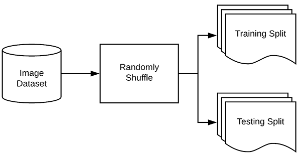
**Figure 5:**在训练深度学习或机器学习模型之前，您必须将数据拆分为训练集和测试集。 这篇博文中使用了 Scikit-learn 来分割我们的数据。

现在我们已经从磁盘加载了我们的图像数据，接下来我们需要构建我们的训练和测试分割：

partition the data into training and testing splits using 75% of

the data for training and the remaining 25% for testing

(trainX, testX, trainY, testY) = train_test_split(data,

labels, test_size=0.25, random_state=42)

按照4：1的比例将数据切分为训练集和测试集。

convert the labels from integers to vectors (for 2-class, binary

classification you should use Keras’ to_categorical function

instead as the scikit-learn’s LabelBinarizer will not return a

vector)

lb = LabelBinarizer()

trainY = lb.fit_transform(trainY)

testY = lb.transform(testY)

将标签做二值化操作

1， 0， 0# 对应猫

0， 1， 0# 对应狗

0， 0， 1# 对应熊猫

请注意，只有一个阵列元素是"hot"的，这就是为什么我们称之为"one-hot"编码。

定义您的 Keras 模型架构

==========================================================================

**图6：**我们简单的神经网络是使用Keras在这个深度学习教程创建的。

下一步是使用 Keras 定义我们的神经网络架构。在这里，我们将使用一个网络，其中一个输入层、两个隐藏层和一个输出层：

define the 3072-1024-512-3 architecture using Keras

model = Sequential()

model.add(Dense(1024, input_shape=(3072,), activation=“sigmoid”))

model.add(Dense(512, activation=“sigmoid”))

model.add(Dense(len(lb.classes_), activation=“softmax”))

由于我们的模型非常简单，我们继续在此脚本中定义它（通常我喜欢在单独的文件中为模型架构创建一个单独的类）。

第一个隐藏层将有节点。input_shape是3072（32x32x3=3072）输出：1024。

第二个隐藏层将有节点输入就是上一个节点的输出所以是1024，输出是512

最后，最终输出层（第 78 行）中的节点数将是可能的类标签的数量——在这种情况下，输出层将有三个节点，一个用于我们的每个类标签（“猫”、“狗” ”和“熊猫”）。

编译你的 Keras 模型

========================================================================

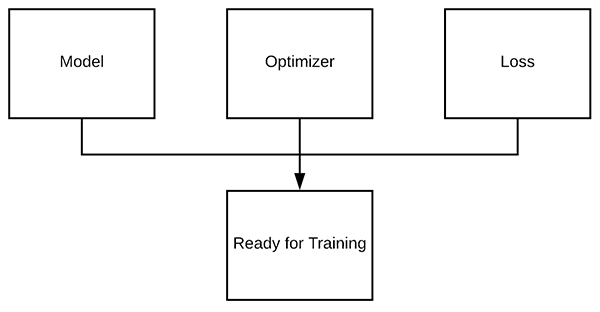
上一步我们定义了我们的神经网络架构，下一步是"compile"它：

initialize our initial learning rate and # of epochs to train for

INIT_LR = 0.01

EPOCHS = 80

compile the model using SGD as our optimizer and categorical

cross-entropy loss (you’ll want to use binary_crossentropy

for 2-class classification)

print(“[INFO] training network…”)

opt = SGD(lr=INIT_LR)

model.compile(loss=“categorical_crossentropy”, optimizer=opt,

metrics=[“accuracy”])

学习率在优化器中设置，优化器使用SGD。

分类交叉熵被用作几乎所有训练进行分类的网络的损失。唯一的例外是_2类分类_，其中只有两个可能的类标签。在这种情况下，你会想交换"categorical_crossentropy"为"binary_crossentropy"。

训练

=============================================================

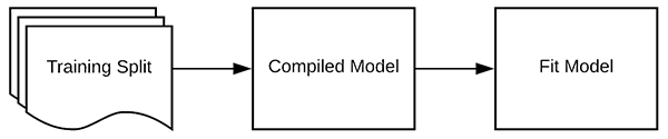
**图8：**训练数据和汇编模型培训深度学习模型。

现在，我们的 Keras 模型已编译，我们可以在我们的培训数据上"拟合"（即训练）它：

train the neural network

H = model.fit(x=trainX, y=trainY, validation_data=(testX, testY),

epochs=EPOCHS, batch_size=32)

batch_size：控制通过网络传递的每组数据的大小。较大的 GPU 将能够容纳更大的批次大小。我建议从32或64（实际大小需要考虑显存的大小）

评估您的Keras模型

======================================================================

[外链图片转存失败,源站可能有防盗链机制,建议将图片保存下来直接上传(img-jOd6McZD-1635420207841)(https://pyimagesearch.com/wp-content/uploads/2018/09/keras_tutorial_step7.png)]

**图9：**在符合我们的模型后，我们可以使用我们的测试数据进行预测并生成分类报告。

我们已经培训了我们的实际模型，但现在我们需要根据我们的测试数据来评估它。

重要的是，我们评估我们的测试数据，以便我们可以获得一个公正的（或尽可能接近公正）的表示，我们的模型如何表现良好的数据，它从来没有受过培训。

evaluate the network

print(“[INFO] evaluating network…”)

predictions = model.predict(x=testX, batch_size=32)

print(classification_report(testY.argmax(axis=1),

predictions.argmax(axis=1), target_names=lb.classes_))

plot the training loss and accuracy

N = np.arange(0, EPOCHS)

plt.style.use(“ggplot”)

plt.figure()

plt.plot(N, H.history[“loss”], label=“train_loss”)

plt.plot(N, H.history[“val_loss”], label=“val_loss”)

plt.plot(N, H.history[“accuracy”], label=“train_acc”)

plt.plot(N, H.history[“val_accuracy”], label=“val_acc”)

plt.title(“Training Loss and Accuracy (Simple NN)”)

plt.xlabel(“Epoch #”)

plt.ylabel(“Loss/Accuracy”)

plt.legend()

plt.savefig(args[“plot”])

运行此脚本时，您会注意到我们的 Keras 神经网络将开始训练，一旦培训完成，我们将评估测试集上的网络：

$ python train_simple_nn.py --dataset animals --model output/simple_nn.model \

–label-bin output/simple_nn_lb.pickle --plot output/simple_nn_plot.png

Using TensorFlow backend.

[INFO] loading images…

[INFO] training network…

Train on 2250 samples, validate on 750 samples

Epoch 1/80

2250/2250 [==============================] - 1s 311us/sample - loss: 1.1041 - accuracy: 0.3516 - val_loss: 1.1578 - val_accuracy: 0.3707

Epoch 2/80

2250/2250 [==============================] - 0s 183us/sample - loss: 1.0877 - accuracy: 0.3738 - val_loss: 1.0766 - val_accuracy: 0.3813

Epoch 3/80

2250/2250 [==============================] - 0s 181us/sample - loss: 1.0707 - accuracy: 0.4240 - val_loss: 1.0693 - val_accuracy: 0.3533

…

Epoch 78/80

2250/2250 [==============================] - 0s 184us/sample - loss: 0.7688 - accuracy: 0.6160 - val_loss: 0.8696 - val_accuracy: 0.5880

Epoch 79/80

2250/2250 [==============================] - 0s 181us/sample - loss: 0.7675 - accuracy: 0.6200 - val_loss: 1.0294 - val_accuracy: 0.5107

Epoch 80/80

2250/2250 [==============================] - 0s 181us/sample - loss: 0.7687 - accuracy: 0.6164 - val_loss: 0.8361 - val_accuracy: 0.6120

[INFO] evaluating network…

precision recall f1-score support

cats 0.57 0.59 0.58 236

dogs 0.55 0.31 0.39 236

panda 0.66 0.89 0.76 278

accuracy 0.61 750

macro avg 0.59 0.60 0.58 750

weighted avg 0.60 0.61 0.59 750

此网络很小，当与小数据集结合时，我的 CPU 上每个epoch只需 2 秒。

在这里你可以看到，我们的网络正在获得60%的准确性。

由于我们随机挑选给定图像的正确标签的几率为 1/3，我们知道我们的网络实际上已经学会了可用于区分三个类别的模式。

我们还保存了我们的情节：

• 训练损失

• 验证损失

• 训练精度

• 验证精度

…确保我们能够轻松地发现我们的结果中过度拟合或不合适。

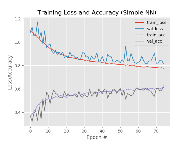
**图10：**我们简单的神经网络训练脚本（与Keras一起创建）生成精确/丢失情节，以帮助我们发现不足/过度拟合。

看看我们的情节，我们看到少量的过度适合开始发生超过epoch+45，我们的训练和验证损失开始分歧，并出现了明显的差距。

最后，我们可以将模型保存到磁盘中，以便以后可以重复使用，而无需重新训练它：

save the model and label binarizer to disk

print(“[INFO] serializing network and label binarizer…”)

model.save(args[“model”], save_format=“h5”)

f = open(args[“label_bin”], “wb”)

f.write(pickle.dumps(lb))

f.close()

使用 Keras 模型对新数据进行预测

==============================================================================

在这一点上， 我们的模型是训练有素的， 但如果我们想在我们的网络已经培训后对图像做出预测呢？

那我们该怎么办？

我们如何从磁盘中加载模型？

我们如何加载图像，然后对图像进行预处理以进行分类？

在predict.py 脚本中，我将向您展示如何操作，因此打开它并插入以下代码：

import the necessary packages

from tensorflow.keras.models import load_model

import argparse

import pickle

import cv2

construct the argument parser and parse the arguments

ap = argparse.ArgumentParser()

ap.add_argument(“-i”, “–image”, required=True,

help=“path to input image we are going to classify”)

ap.add_argument(“-m”, “–model”, required=True,

help=“path to trained Keras model”)

ap.add_argument(“-l”, “–label-bin”, required=True,

help=“path to label binarizer”)

ap.add_argument(“-w”, “–width”, type=int, default=28,

help=“target spatial dimension width”)

ap.add_argument(“-e”, “–height”, type=int, default=28,

help=“target spatial dimension height”)

ap.add_argument(“-f”, “–flatten”, type=int, default=-1,

help=“whether or not we should flatten the image”)

args = vars(ap.parse_args())

首先，我们将导入所需的包和模块。 每当您编写脚本以从磁盘加载 Keras 模型时，您都需要显式导入 from。 OpenCV 将用于注释和显示。该模块将用于加载我们的标签 binarizer.load_modeltensorflow.keras.modelspickle 接下来，让我们解析我们的命令行参数：

–image ：我们输入图像的路径。

–model ：我们经过训练和序列化的 Keras 模型路径。

–label-bin ：序列化标签二值化器的路径。

–width ：我们的 CNN 输入形状的宽度。本次设置为32。

–height ：输入到 CNN 的图像的高度。本次设置为32。

–flatten ：我们是否应该展平图像。默认情况下，我们不会展平图像。如果您需要展平图像，将其设置为1。

接下来，让我们根据命令行参数加载图像并调整其大小：

load the input image and resize it to the target spatial dimensions

image = cv2.imread(args[“image”])

output = image.copy()

image = cv2.resize(image, (args[“width”], args[“height”]))

scale the pixel values to [0, 1]

image = image.astype(“float”) / 255.0

check to see if we should flatten the image and add a batch

dimension

if args[“flatten”] > 0:

image = image.flatten()

image = image.reshape((1, image.shape[0]))

otherwise, we must be working with a CNN – don’t flatten the

image, simply add the batch dimension

else:

image = image.reshape((1, image.shape[0], image.shape[1],

image.shape[2]))

将图像展平。

load the model and label binarizer

print(“[INFO] loading network and label binarizer…”)

model = load_model(args[“model”])

lb = pickle.loads(open(args[“label_bin”], “rb”).read())

make a prediction on the image

preds = model.predict(image)

find the class label index with the largest corresponding

probability

i = preds.argmax(axis=1)[0]

label = lb.classes_[i]

加载模型然后预测模型

• 猫： 54.6%

• 狗： 45.4%

• 熊猫： +0%

换句话说，我们的网络"认为"它看到*“猫”，它肯定"知道"它没有看到"熊猫"。*

找到最大值的索引（第 0 个"猫"指数）。

标签二进制器中提取‘“猫”字符串标签。

很简单， 对吧？

现在，让我们显示结果：

draw the class label + probability on the output image

text = “{}: {:.2f}%”.format(label, preds[0][i] * 100)

cv2.putText(output, text, (10, 30), cv2.FONT_HERSHEY_SIMPLEX, 0.7,

(0, 0, 255), 2)

show the output image

cv2.imshow(“Image”, output)

cv2.waitKey(0)

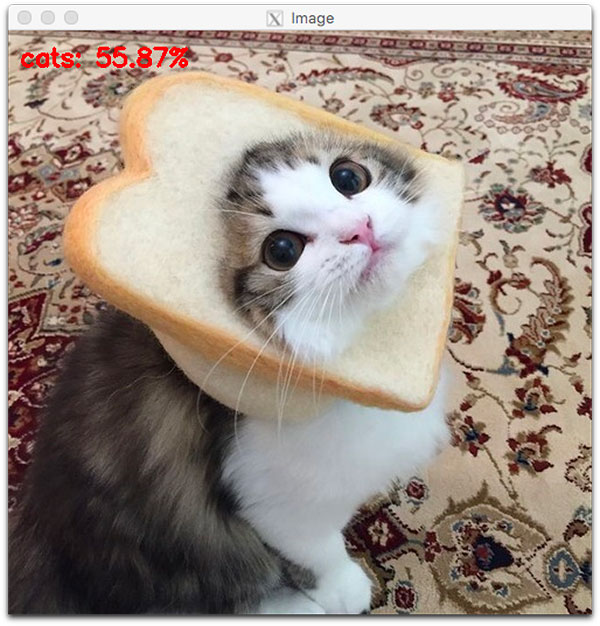
**图11：**在我们的 Keras 教程中，猫被正确地分类为一个简单的神经网络。

在这里你可以看到，我们简单的Keras神经网络已经分类输入图像为"猫"55.87%的概率，尽管猫的脸被一块面包部分遮盖。

搭建CNN网络

==================================================================

无可否认，使用标准的馈入神经网络对图像进行分类并不是一个明智的选择。

相反，我们应该利用卷积神经网络 （CNN），该网络旨在对图像的原始像素强度进行操作，并学习可用于高精度对图像进行分类的歧视性滤镜。

我们今天在这里讨论的模型是Vggnet的较小变体， 我称之为 “小 Vggnet” 。

VGGNet 样型号具有两个共同特征：

1. 只使用 3×3 卷积核

2. 在应用池操作之前，在网络架构中，相互叠加在一起

现在，让我们继续实施小型VGGNet。

打开

smallvggnet.py

文件并插入以下代码：

import the necessary packages

from tensorflow.keras.models import Sequential

from tensorflow.keras.layers import BatchNormalization

from tensorflow.keras.layers import Conv2D

from tensorflow.keras.layers import MaxPooling2D

from tensorflow.keras.layers import Activation

from tensorflow.keras.layers import Flatten

from tensorflow.keras.layers import Dropout

from tensorflow.keras.layers import Dense

from tensorflow.keras import backend as K

导入需要的包。

class SmallVGGNet:

@staticmethod

def build(width, height, depth, classes):

initialize the model along with the input shape to be

“channels last” and the channels dimension itself

model = Sequential()

inputShape = (height, width, depth)

chanDim = -1

if we are using “channels first”, update the input shape

and channels dimension

if K.image_data_format() == “channels_first”:

inputShape = (depth, height, width)

chanDim = 1

创建SmallVGGNet类，在类中增加build方法。

build需要四个参数，分别是宽，高，深度和类别。

CONV => RELU => POOL layer set

model.add(Conv2D(32, (3, 3), padding=“same”,

input_shape=inputShape))

model.add(Activation(“relu”))

model.add(BatchNormalization(axis=chanDim))

model.add(MaxPooling2D(pool_size=(2, 2)))

model.add(Dropout(0.25))

第一个卷积层，经过池化后，尺寸减少一半。

(CONV => RELU) * 2 => POOL layer set

model.add(Conv2D(64, (3, 3), padding=“same”))

model.add(Activation(“relu”))

model.add(BatchNormalization(axis=chanDim))

model.add(Conv2D(64, (3, 3), padding=“same”))

model.add(Activation(“relu”))

model.add(BatchNormalization(axis=chanDim))

model.add(MaxPooling2D(pool_size=(2, 2)))

model.add(Dropout(0.25))

第二个卷积层，经过池化后，尺寸减少一半。

(CONV => RELU) * 3 => POOL layer set

model.add(Conv2D(128, (3, 3), padding=“same”))

model.add(Activation(“relu”))

model.add(BatchNormalization(axis=chanDim))

model.add(Conv2D(128, (3, 3), padding=“same”))

model.add(Activation(“relu”))

model.add(BatchNormalization(axis=chanDim))

model.add(Conv2D(128, (3, 3), padding=“same”))

model.add(Activation(“relu”))

model.add(BatchNormalization(axis=chanDim))

model.add(MaxPooling2D(pool_size=(2, 2)))

model.add(Dropout(0.25))

第三个卷积层，经过池化后，尺寸减少一半。

first (and only) set of FC => RELU layers

model.add(Flatten())

model.add(Dense(512))

model.add(Activation(“relu”))

model.add(BatchNormalization())

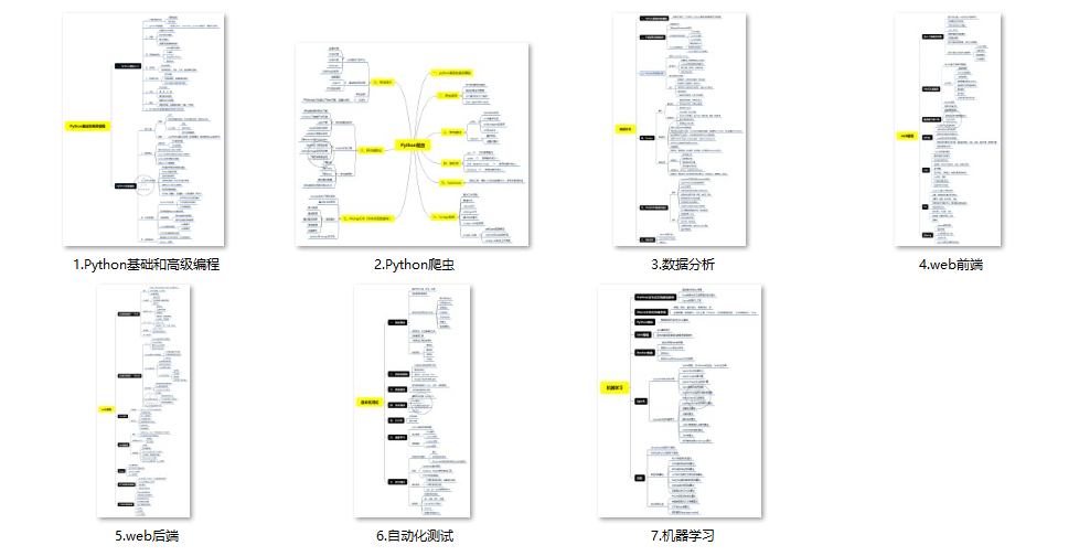
（1）Python所有方向的学习路线（新版）

这是我花了几天的时间去把Python所有方向的技术点做的整理，形成各个领域的知识点汇总，它的用处就在于，你可以按照上面的知识点去找对应的学习资源，保证自己学得较为全面。

最近我才对这些路线做了一下新的更新，知识体系更全面了。

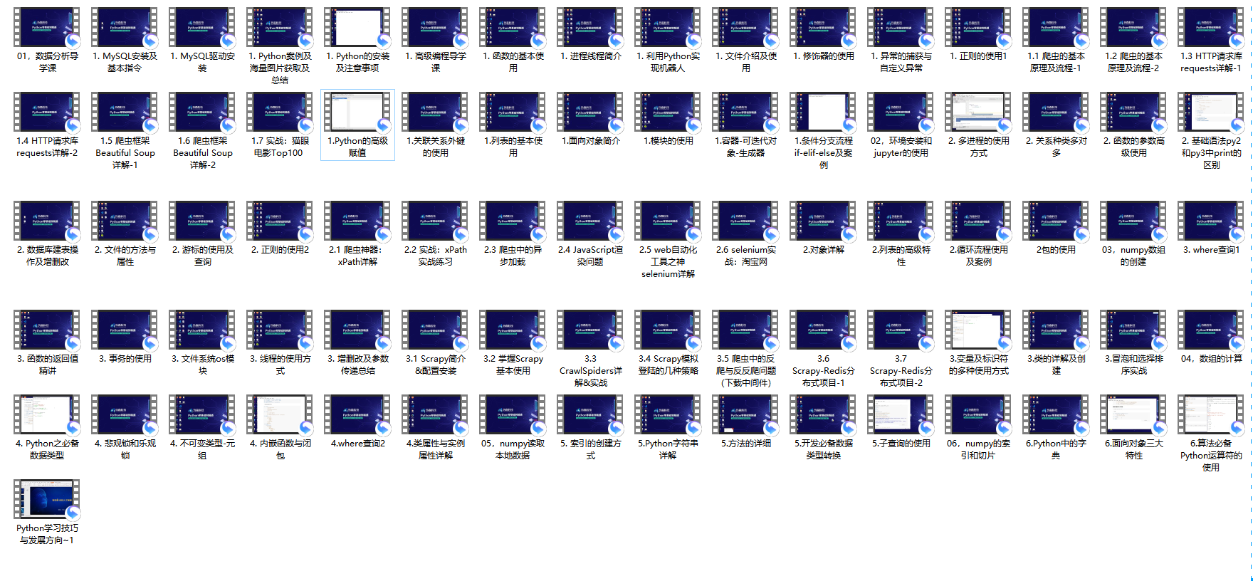
（2）Python学习视频

包含了Python入门、爬虫、数据分析和web开发的学习视频，总共100多个，虽然没有那么全面，但是对于入门来说是没问题的，学完这些之后，你可以按照我上面的学习路线去网上找其他的知识资源进行进阶。

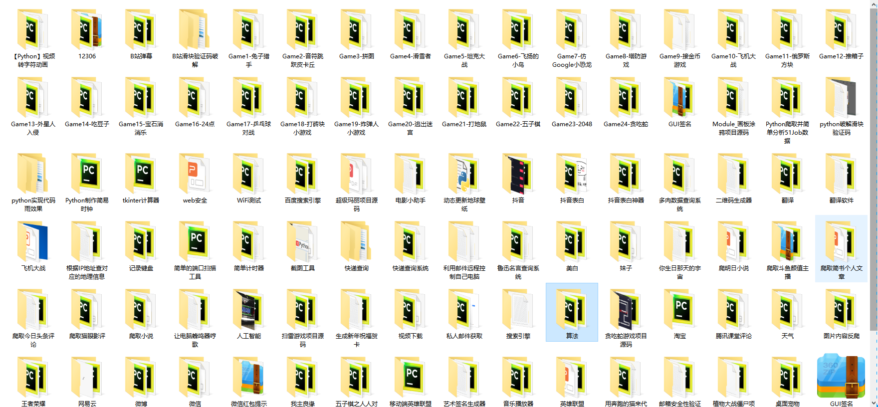
（3）100多个练手项目

我们在看视频学习的时候，不能光动眼动脑不动手，比较科学的学习方法是在理解之后运用它们，这时候练手项目就很适合了，只是里面的项目比较多，水平也是参差不齐，大家可以挑自己能做的项目去练练。

网上学习资料一大堆，但如果学到的知识不成体系，遇到问题时只是浅尝辄止，不再深入研究，那么很难做到真正的技术提升。

需要这份系统化学习资料的朋友，可以戳这里无偿获取

一个人可以走的很快，但一群人才能走的更远！不论你是正从事IT行业的老鸟或是对IT行业感兴趣的新人，都欢迎加入我们的的圈子（技术交流、学习资源、职场吐槽、大厂内推、面试辅导），让我们一起学习成长！