


DAY 32 官方文档的阅读
知识点回顾:
- 官方文档的检索方式:github和官网
- 官方文档的阅读和使用:要求安装的包和文档为同一个版本
- 类的关注点:
- 实例化所需要的参数
- 普通方法所需要的参数
- 普通方法的返回值
- 绘图的理解:对底层库的调用
作业:参考pdpbox官方文档中的其他类,绘制相应的图,任选即可
import pandas as pd
from sklearn.datasets import load_iris
from sklearn.model_selection import train_test_split
from sklearn.ensemble import RandomForestClassifier

# 加载鸢尾花数据集
iris = load_iris()
df = pd.DataFrame(iris.data, columns=iris.feature_names)
df['target'] = iris.target  # 添加目标列(0-2类:山鸢尾、杂色鸢尾、维吉尼亚鸢尾)

# 特征与目标变量
features = iris.feature_names  # 4个特征:花萼长度、花萼宽度、花瓣长度、花瓣宽度
target = 'target'  # 目标列名

# 划分训练集与测试集
X_train, X_test, y_train, y_test = train_test_split(
    df[features], df[target], test_size=0.2, random_state=42
)

# 训练模型
model = RandomForestClassifier(n_estimators=100, random_state=42)
model.fit(X_train, y_train)

# 首先要确保库的版本是最新的,因为我们看的是最新的文档,库的版本可以在github上查看
import  pdpbox
print(pdpbox.__version__)  # pdpbox版本

#InteractTargetPlot
from pdpbox.info_plots import InteractTargetPlot
features = 'petal length (cm)','petal width (cm)'  # 要分析的特征
feature_names = features
# 绘制交互目标图
Interact_TargetPlot = InteractTargetPlot(
    df =df,  # 数据集
    features = features,
    feature_names = feature_names,  # 特征名称
    target = target,  # 目标变量
    num_grid_points = 10,  # 网格点数量
    grid_types = 'percentile',  # 网格类型
)
Interact_TargetPlot.plot()
type(Interact_TargetPlot.plot())
len(Interact_TargetPlot.plot())
Interact_TargetPlot.plot()[0]
Interact_TargetPlot.plot()[1]
Interact_TargetPlot.plot()[2]

fig,axes,summary_df = Interact_TargetPlot.plot(
    which_classes=None,  # 绘制所有类别(0,1,2)
    show_percentile=True,  # 显示百分位线
    engine='plotly',
    template='plotly_white'
)  # 绘制交互目标图,并返回fig,axes,summary_df
# 手动设置图表尺寸(单位:像素)
fig.update_layout(
    width=800,  # 宽度800像素
    height=500,  # 高度500像素
    title=dict(text=f'InteractTarget Plot: {feature_name}', x=0.5)  # 居中标题
)

fig.show()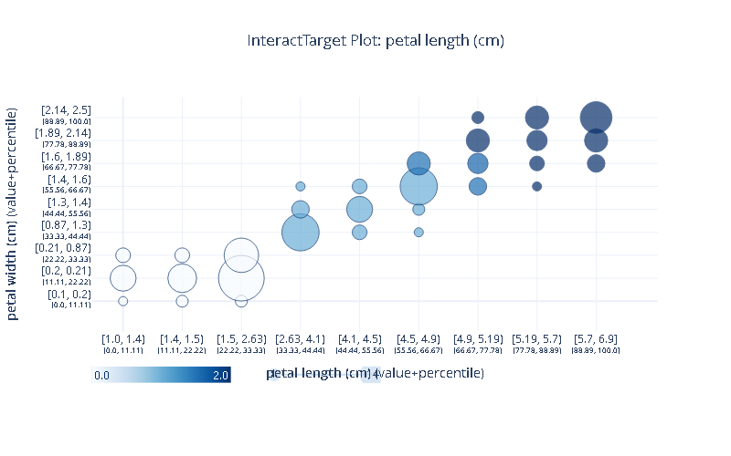
#PredictPlot
from pdpbox.info_plots import PredictPlot
feature = 'petal length (cm)' # 要分析的特征
feature_name = feature
# 绘制预测图
Predict_Plot = PredictPlot(
    df = df,  # 数据集
    feature = feature,  # 要分析的特征
    feature_name = feature_name,  # 特征名称
    model = model,  # 训练好的模型
    num_grid_points = 10,  # 网格点数量
    grid_type = 'percentile',  # 网格类型
    model_features = features,  # 模型使用的特征
)
Predict_Plot.plot()  # 绘制预测图
fig,axes,summary_df = Predict_Plot.plot(
    which_classes=None,  # 绘制所有类别(0,1,2)
    show_percentile=True,  # 显示百分位线
    engine='plotly',
    template='plotly_white'
)
fig.update_layout(
    width=1000,  # 宽度800像素
    height=1400,  # 高度500像素
    title=dict(text=f'Predict Plot: {feature_name}', x=0.5)  # 居中标题
)
fig.show()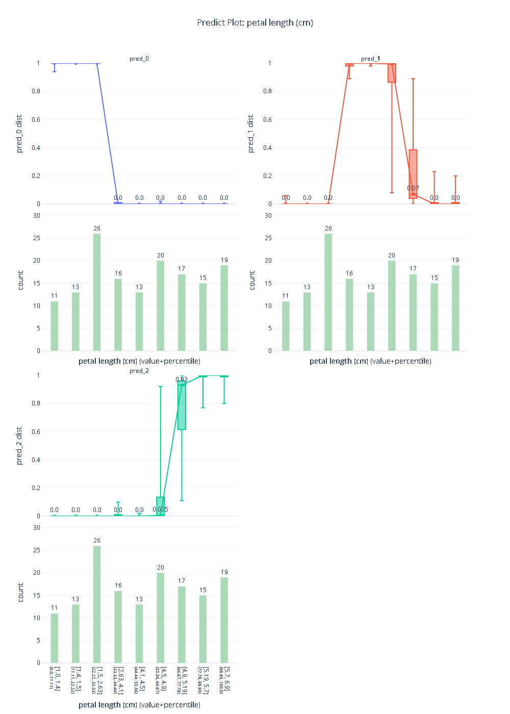
#PDPIsolate
from pdpbox.pdp import PDPIsolate
feature = 'petal length (cm)'  # 要分析的特征
feature_name = feature
# 计算PDP
PDP_Isolate = PDPIsolate(
    model = model,  # 训练好的模型
    df = df,  # 数据集
    model_features = features,  # 模型使用的特征
    feature = feature,  # 要分析的特征
    feature_name = feature_name,  # 特征名称
    num_grid_points = 10,  # 网格点数量
    grid_type = 'percentile',  # 网格类型
    )

PDP_Isolate.plot()  # 绘制PDP
type(PDP_Isolate.plot())  # 查看返回值类型
len(PDP_Isolate.plot())  # 查看返回值长度
PDP_Isolate.plot()[0]  # 查看第一个返回值
PDP_Isolate.plot()[1]  # 查看第二个返回值

fig,axes = PDP_Isolate.plot(
    which_classes=None,  # 绘制所有类别(0,1,2)
    show_percentile=True,  # 显示百分位线
    engine='plotly',
    template='plotly_white'
    )
fig.update_layout(
    width=1000,  # 宽度800像素
    height=1000,  # 高度500像素
    title=dict(text=f'Predict Plot: {feature_name}', x=0.5)  # 居中标题
)
fig.show()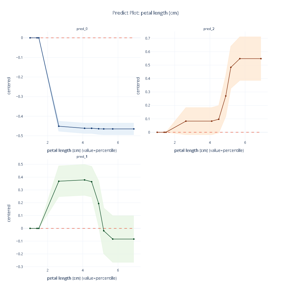


 263
263

 被折叠的 条评论
为什么被折叠?
被折叠的 条评论
为什么被折叠?
 到【灌水乐园】发言


