5月12日day23打卡

pipeline管道

知识回顾:

1. 转化器和估计器的概念
2. 管道工程
3. ColumnTransformer和Pipeline类

作业：

整理下全部逻辑的先后顺序，看看能不能制作出适合所有机器学习的通用pipeline

基础概念

 pipeline在机器学习领域可以翻译为“管道”，也可以翻译为“流水线”，是机器学习中一个重要的概
念。

在机器学习中，通常会按照一定的顺序对数据进行预处理、特征提取、模型训练和模型评估等步骤，以实现机器学习模型的训练和评估。为了方便管理这些步骤，我们可以使用pipeline来构建个完整的机器学习流水线。

pipeline是一个用于组合多个估计器(estimator)的estimator,.它实现了一个流水线，其中每个估计器都按照一定的顺序执行。在pipelinet中，每个估计器都实现了fit和transform方法，fit方法用于训练模型，transform方法用于对数据进行预处理和特征提取。

在此之前我们先介绍下转换器(transformer)和估计器(estimator)的概念。

转换器(transformer) 

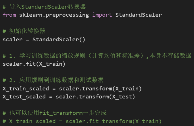
转换器(transformer）)是一个用于对数据进行预处理和特征提取的estimator,它实现一个transform方法，用于对数据进行预处理和特征提取。转换器通常用于对数据进行预处理，例如对数据进行归一化、标准化、缺失值填充等。转换器也可以用于对数据进行特征提取，例如对数据进行特征选择、特征组合等。转换器的特点是无状态的，即它们不会存储任何关于数据的状态信息（指的是不存储内参）。转换器仅根据输入数据学习转换规则（比如函数规律、外参），并将其应用于新的数据。因此，转换器可以在训练集上学习转换规则，并在训练集之外的新数据上应用这些规则。

常见的转换器包括数据缩放器（如StandardScaler、MinMaxScaler)、特征选择器(如SelectKBest、PCA)、特征提取器（如CountVectorizer、TF-IDFVectorizer))等。

之前我们都是说对xxxx类进行实例化，现在可以换一个更加准确的说法，如下： 

 

 估计器(estimator)

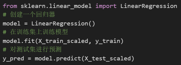
估计器(Estimator）是实现机器学习算法的对象或类。它用于拟合(fit)数据并进行预测(predict)。估计器是机器学习模型的基本组成部分，用于从数据中学习模式、进行预测和进行模型评估。 

估计器的主要方法是fit和predict。.fit方法用于根据输入数据学习模型的参数和规律，而predict方法用于对新的未标记样本进行预测。估计器的特点是有状态的，即它们在训练过程中存储了关于数据的状态信息，以便在预测阶段使用。估计器通过学习训练数据中的模式和规律来进行预测。因此，估计器需要在训练集上进行训练，并使用训练得到的模型参数对新数据进行预测。

常见的估计器包括分类器(classifier）)、回归器(regresser)、聚类器(clusterer)。 

 

管道(pipeline)

了解了分类器和估计器，所以可以理解为在机器学习是由转换器(Transformer))和估计器(Estimator))按照一定顺序组合在一起的来完成了整个流程。

机器学习的管道(Pipeline)机制通过将多个转换器和估计器按顺序连接在一起，可以构建一个完整的数据处理和模型训练流程。在管道机制中，可以使用Pipeline类来组织和连接不同的转换器和估计器。Pipeline类提供了一种简单的方式来定义和管理机器学习任务的流程。

管道机制是按照封装顺序依次执行的一种机制，在机器学习算法中得以应用的根源在于，参数集在新数据集（比如测试集）上的重复使用。且代码看上去更加简洁明确。这也意味着，很多个不同的数据集，只要处理成管道的输入形式，后续的代码就可以复用。（这里为我们未来的oythor文件拆分做铺垫)，也就是把很多个类和函数操作写进一个新的pipeline中。

这符合编程中的一个非常经典的思想：don't repeat yourself。(dry原则)，也叫做封装思想，我们之前提到过类似的思想的应用：函数、类，现在我们来说管道。

Pipelinef最大的价值和核心应用场景之一，就是与交叉验证和网格搜索等结合使用，来：

1. 防止数据泄露：这是在使用交叉验证时，Pipeline自动完成预处理并在每个折叠内独立fit/transform的关键优势。
2. 简化超参数调优：可以方便地同时调优预处理步骤和模型的参数。

下面我们将对我们的信贷数据集进行管道工程，重构整个代码。之所以提到管道，是因为后续你在阅读一些经典的代码的时候，尤其是官方文档，非常喜欢用管道来构建代码，甚至深度学习中也有类似的代码，初学者往往看起来很吃力。

代码演示

没有pipline的代码
 

# 先运行之前预处理好的代码
import pandas as pd
import pandas as pd    #用于数据处理和分析，可处理表格数据。
import numpy as np     #用于数值计算，提供了高效的数组操作。
import matplotlib.pyplot as plt    #用于绘制各种类型的图表
import seaborn as sns   #基于matplotlib的高级绘图库，能绘制更美观的统计图形。
import warnings
warnings.filterwarnings("ignore")
 
 # 设置中文字体（解决中文显示问题）
plt.rcParams['font.sans-serif'] = ['SimHei']  # Windows系统常用黑体字体
plt.rcParams['axes.unicode_minus'] = False    # 正常显示负号
data = pd.read_csv('data.csv')    #读取数据


# 先筛选字符串变量 
discrete_features = data.select_dtypes(include=['object']).columns.tolist()
# Home Ownership 标签编码
home_ownership_mapping = {
    'Own Home': 1,
    'Rent': 2,
    'Have Mortgage': 3,
    'Home Mortgage': 4
}
data['Home Ownership'] = data['Home Ownership'].map(home_ownership_mapping)

# Years in current job 标签编码
years_in_job_mapping = {
    '< 1 year': 1,
    '1 year': 2,
    '2 years': 3,
    '3 years': 4,
    '4 years': 5,
    '5 years': 6,
    '6 years': 7,
    '7 years': 8,
    '8 years': 9,
    '9 years': 10,
    '10+ years': 11
}
data['Years in current job'] = data['Years in current job'].map(years_in_job_mapping)

# Purpose 独热编码，记得需要将bool类型转换为数值
data = pd.get_dummies(data, columns=['Purpose'])
data2 = pd.read_csv("data.csv") # 重新读取数据，用来做列名对比
list_final = [] # 新建一个空列表，用于存放独热编码后新增的特征名
for i in data.columns:
    if i not in data2.columns:
       list_final.append(i) # 这里打印出来的就是独热编码后的特征名
for i in list_final:
    data[i] = data[i].astype(int) # 这里的i就是独热编码后的特征名



# Term 0 - 1 映射
term_mapping = {
    'Short Term': 0,
    'Long Term': 1
}
data['Term'] = data['Term'].map(term_mapping)
data.rename(columns={'Term': 'Long Term'}, inplace=True) # 重命名列
continuous_features = data.select_dtypes(include=['int64', 'float64']).columns.tolist()  #把筛选出来的列名转换成列表
 
 # 连续特征用中位数补全
for feature in continuous_features:     
    mode_value = data[feature].mode()[0]            #获取该列的众数。
    data[feature].fillna(mode_value, inplace=True)          #用众数填充该列的缺失值，inplace=True表示直接在原数据上修改。

# 最开始也说了 很多调参函数自带交叉验证，甚至是必选的参数，你如果想要不交叉反而实现起来会麻烦很多
# 所以这里我们还是只划分一次数据集
from sklearn.model_selection import train_test_split
X = data.drop(['Credit Default'], axis=1)  # 特征，axis=1表示按列删除
y = data['Credit Default'] # 标签
# 按照8:2划分训练集和测试集
X_train, X_test, y_train, y_test = train_test_split(X, y, test_size=0.2, random_state=42)  # 80%训练集，20%测试集


from sklearn.ensemble import RandomForestClassifier #随机森林分类器

from sklearn.metrics import accuracy_score, precision_score, recall_score, f1_score # 用于评估分类器性能的指标
from sklearn.metrics import classification_report, confusion_matrix #用于生成分类报告和混淆矩阵
import warnings #用于忽略警告信息
warnings.filterwarnings("ignore") # 忽略所有警告信息
# --- 1. 默认参数的随机森林 ---
# 评估基准模型，这里确实不需要验证集
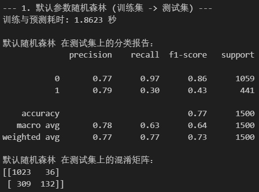
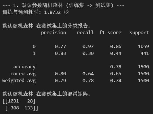
print("--- 1. 默认参数随机森林 (训练集 -> 测试集) ---")
import time # 这里介绍一个新的库，time库，主要用于时间相关的操作，因为调参需要很长时间，记录下会帮助后人知道大概的时长
start_time = time.time() # 记录开始时间
rf_model = RandomForestClassifier(random_state=42)
rf_model.fit(X_train, y_train) # 在训练集上训练
rf_pred = rf_model.predict(X_test) # 在测试集上预测
end_time = time.time() # 记录结束时间

print(f"训练与预测耗时: {end_time - start_time:.4f} 秒")
print("\n默认随机森林 在测试集上的分类报告：")
print(classification_report(y_test, rf_pred))
print("默认随机森林 在测试集上的混淆矩阵：")
print(confusion_matrix(y_test, rf_pred))

 

pipelinel的代码教学 

 导入库和数据加载

# 导入基础库
import pandas as pd
import numpy as np
import matplotlib.pyplot as plt
import seaborn as sns
import time # 导入 time 库
import warnings

# 忽略警告
warnings.filterwarnings("ignore")

# 设置中文字体和负号正常显示
plt.rcParams['font.sans-serif'] = ['SimHei']
plt.rcParams['axes.unicode_minus'] = False

# 导入 Pipeline 和相关预处理工具
from sklearn.pipeline import Pipeline # 用于创建机器学习工作流
from sklearn.compose import ColumnTransformer # 用于将不同的预处理应用于不同的列
from sklearn.preprocessing import OrdinalEncoder, OneHotEncoder, StandardScaler # 用于数据预处理（有序编码、独热编码、标准化）
from sklearn.impute import SimpleImputer # 用于处理缺失值

# 导入机器学习模型和评估工具
from sklearn.ensemble import RandomForestClassifier # 随机森林分类器
from sklearn.metrics import classification_report, confusion_matrix # 用于评估分类器性能
from sklearn.model_selection import train_test_split # 用于划分训练集和测试集


# --- 加载原始数据 ---
# 我们加载原始数据，不对其进行任何手动预处理
data = pd.read_csv('data.csv')

print("原始数据加载完成，形状为:", data.shape)
# print(data.head()) # 可以打印前几行看看原始数据

分离特征和标签，划分数据集

# --- 分离特征和标签 (使用原始数据) ---
y = data['Credit Default'] # 标签
X = data.drop(['Credit Default'], axis=1) # 特征 (axis=1 表示按列删除)

print("\n特征和标签分离完成。")
print("特征 X 的形状:", X.shape)
print("标签 y 的形状:", y.shape)

# --- 划分训练集和测试集 (在任何预处理之前划分) ---
# 按照8:2划分训练集和测试集
X_train, X_test, y_train, y_test = train_test_split(X, y, test_size=0.2, random_state=42) # 80%训练集，20%测试集

print("\n数据集划分完成 (预处理之前)。")
print("X_train 形状:", X_train.shape)
print("X_test 形状:", X_test.shape)
print("y_train 形状:", y_train.shape)
print("y_test 形状:", y_test.shape)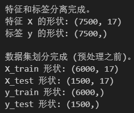

 定义预处理步骤

ColumTransformerl的核心 

# --- 定义不同列的类型和它们对应的预处理步骤 ---
# 这些定义是基于原始数据 X 的列类型来确定的

# 识别原始的 object 列 (对应你原代码中的 discrete_features 在预处理前)
object_cols = X.select_dtypes(include=['object']).columns.tolist()
# 识别原始的非 object 列 (通常是数值列)
numeric_cols = X.select_dtypes(exclude=['object']).columns.tolist()


# 有序分类特征 (对应你之前的标签编码)
# 注意：OrdinalEncoder默认编码为0, 1, 2... 对应你之前的1, 2, 3...需要在模型解释时注意
# 这里的类别顺序需要和你之前映射的顺序一致
ordinal_features = ['Home Ownership', 'Years in current job', 'Term']
# 定义每个有序特征的类别顺序，这个顺序决定了编码后的数值大小
ordinal_categories = [
    ['Own Home', 'Rent', 'Have Mortgage', 'Home Mortgage'], # Home Ownership 的顺序 (对应1, 2, 3, 4)
    ['< 1 year', '1 year', '2 years', '3 years', '4 years', '5 years', '6 years', '7 years', '8 years', '9 years', '10+ years'], # Years in current job 的顺序 (对应1-11)
    ['Short Term', 'Long Term'] # Term 的顺序 (对应0, 1)
]
# 构建处理有序特征的 Pipeline: 先填充缺失值，再进行有序编码
ordinal_transformer = Pipeline(steps=[
    ('imputer', SimpleImputer(strategy='most_frequent')), # 用众数填充分类特征的缺失值
    ('encoder', OrdinalEncoder(categories=ordinal_categories, handle_unknown='use_encoded_value', unknown_value=-1)) # 进行有序编码
])
print("有序特征处理 Pipeline 定义完成。")


# 标称分类特征 (对应你之前的独热编码)
nominal_features = ['Purpose'] # 使用原始列名
# 构建处理标称特征的 Pipeline: 先填充缺失值，再进行独热编码
nominal_transformer = Pipeline(steps=[
    ('imputer', SimpleImputer(strategy='most_frequent')), # 用众数填充分类特征的缺失值
    ('onehot', OneHotEncoder(handle_unknown='ignore', sparse_output=False)) # 进行独热编码, sparse_output=False 使输出为密集数组
])
print("标称特征处理 Pipeline 定义完成。")


# 连续特征 (对应你之前的众数填充 + 添加标准化)
# 从所有列中排除掉分类特征，得到连续特征列表
# continuous_features = X.columns.difference(object_cols).tolist() # 原始X中非object类型的列
# 也可以直接从所有列中排除已知的有序和标称特征
continuous_features = [f for f in X.columns if f not in ordinal_features + nominal_features]

# 构建处理连续特征的 Pipeline: 先填充缺失值，再进行标准化
continuous_transformer = Pipeline(steps=[
    ('imputer', SimpleImputer(strategy='most_frequent')), # 用众数填充缺失值 (复现你的原始逻辑)
    ('scaler', StandardScaler()) # 标准化，一个好的实践 (如果你严格复刻原代码，可以移除这步)
])
print("连续特征处理 Pipeline 定义完成。")

 

# --- 构建 ColumnTransformer ---
# 将不同的预处理应用于不同的列子集，构造一个完备的转化器
# ColumnTransformer 接收一个 transformers 列表，每个元素是 (名称, 转换器对象, 列名列表)
preprocessor = ColumnTransformer(
    transformers=[
        ('ordinal', ordinal_transformer, ordinal_features), # 对 ordinal_features 列应用 ordinal_transformer
        ('nominal', nominal_transformer, nominal_features), # 对 nominal_features 列应用 nominal_transformer
        ('continuous', continuous_transformer, continuous_features) # 对 continuous_features 列应用 continuous_transformer
    ],
    remainder='passthrough' # 如何处理没有在上面列表中指定的列。
                           # 'passthrough' 表示保留这些列，不做任何处理。
                           # 'drop' 表示丢弃这些列。
)

print("\nColumnTransformer (预处理器) 定义完成。")
# print(preprocessor) # 可以打印 preprocessor 对象看看它的结构

 

 构建完整pipeline

# --- 构建完整的 Pipeline ---
# 将预处理器和模型串联起来
# 使用你原代码中 RandomForestClassifier 的默认参数和 random_state
pipeline = Pipeline(steps=[
    ('preprocessor', preprocessor), # 第一步：应用所有的预处理 (我们刚刚定义的 ColumnTransformer 对象)
    ('classifier', RandomForestClassifier(random_state=42)) # 第二步：随机森林分类器 (使用默认参数和指定的 random_state)
])

print("\n完整的 Pipeline 定义完成。")
# print(pipeline) # 可以打印 pipeline 对象看看它的结构

 

使用Pipeline进行训练和评估

# --- 1. 使用 Pipeline 在划分好的训练集和测试集上评估 ---
# 完全模仿你原代码的第一个评估步骤

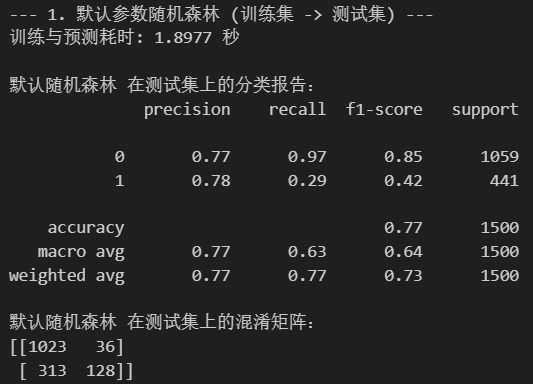
print("\n--- 1. 默认参数随机森林 (训练集 -> 测试集) ---") # 使用你原代码的输出文本
# import time # 引入 time 库 (已在文件顶部引入)

start_time = time.time() # 记录开始时间

# 在原始的 X_train, y_train 上拟合整个Pipeline
# Pipeline会自动按顺序执行 preprocessor 的 fit_transform(X_train)，
# 然后用处理后的数据和 y_train 拟合 classifier
pipeline.fit(X_train, y_train)

# 在原始的 X_test 上进行预测
# Pipeline会自动按顺序执行 preprocessor 的 transform(X_test)，
# 然后用处理后的数据进行 classifier 的 predict
pipeline_pred = pipeline.predict(X_test)

end_time = time.time() # 记录结束时间

print(f"训练与预测耗时: {end_time - start_time:.4f} 秒") # 使用你原代码的输出格式

print("\n默认随机森林 在测试集上的分类报告：") # 使用你原代码的输出文本
print(classification_report(y_test, pipeline_pred))
print("默认随机森林 在测试集上的混淆矩阵：") # 使用你原代码的输出文本
print(confusion_matrix(y_test, pipeline_pred))

 

代码汇总 

import pandas as pd
import numpy as np
import matplotlib.pyplot as plt
import seaborn as sns
import time # 导入 time 库
import warnings
warnings.filterwarnings("ignore")
plt.rcParams['font.sans-serif'] = ['SimHei']
plt.rcParams['axes.unicode_minus'] = False # 防止负号显示问题

# 导入 Pipeline 和相关预处理工具
from sklearn.pipeline import Pipeline #  用于创建机器学习工作流
from sklearn.compose import ColumnTransformer # 用于将不同的预处理应用于不同的列，之前是对datafame的某一列手动处理，如果在pipeline中直接用standardScaler等函数就会对所有列处理，所以要用到这个工具
from sklearn.preprocessing import OrdinalEncoder, OneHotEncoder, StandardScaler # 用于数据预处理
from sklearn.impute import SimpleImputer # 用于处理缺失值

# 机器学习相关库
from sklearn.ensemble import RandomForestClassifier
from sklearn.metrics import classification_report, confusion_matrix, accuracy_score, precision_score, recall_score, f1_score
from sklearn.model_selection import train_test_split # 只导入 train_test_split


# --- 加载原始数据 ---
data = pd.read_csv('data.csv')


# Pipeline 将直接处理分割后的原始数据 X_train, X_test
# 原手动预处理步骤 (将被Pipeline替代):
# Home Ownership 标签编码
# Years in current job 标签编码
# Purpose 独热编码
# Term 0 - 1 映射并重命名
# 连续特征用众数补全


# --- 分离特征和标签 (使用原始数据) ---
y = data['Credit Default']
X = data.drop(['Credit Default'], axis=1)

# --- 划分训练集和测试集 (在任何预处理之前划分) ---
# X_train 和 X_test 现在是原始数据中划分出来的部分，不包含你之前的任何手动预处理结果
X_train, X_test, y_train, y_test = train_test_split(X, y, test_size=0.2, random_state=42)


# --- 定义不同列的类型和它们对应的预处理步骤 (这些将被放入 Pipeline 的 ColumnTransformer 中) ---
# 这些定义是基于原始数据 X 的列类型来确定的

# 识别原始的 object 列 (对应你原代码中的 discrete_features 在预处理前)
object_cols = X.select_dtypes(include=['object']).columns.tolist()

# 有序分类特征 (对应你之前的标签编码)
# 注意：OrdinalEncoder默认编码为0, 1, 2... 对应你之前的1, 2, 3...需要在模型解释时注意
# 这里的类别顺序需要和你之前映射的顺序一致
ordinal_features = ['Home Ownership', 'Years in current job', 'Term']
# 定义每个有序特征的类别顺序，这个顺序决定了编码后的数值大小
ordinal_categories = [
    ['Own Home', 'Rent', 'Have Mortgage', 'Home Mortgage'], # Home Ownership 的顺序 (对应1, 2, 3, 4)
    ['< 1 year', '1 year', '2 years', '3 years', '4 years', '5 years', '6 years', '7 years', '8 years', '9 years', '10+ years'], # Years in current job 的顺序 (对应1-11)
    ['Short Term', 'Long Term'] # Term 的顺序 (对应0, 1)
]
# 先用众数填充分类特征的缺失值，然后进行有序编码
ordinal_transformer = Pipeline(steps=[
    ('imputer', SimpleImputer(strategy='most_frequent')), # 用众数填充分类特征的缺失值
    ('encoder', OrdinalEncoder(categories=ordinal_categories, handle_unknown='use_encoded_value', unknown_value=-1))
])


# 分类特征 
nominal_features = ['Purpose'] # 使用原始列名
# 先用众数填充分类特征的缺失值，然后进行独热编码
nominal_transformer = Pipeline(steps=[
    ('imputer', SimpleImputer(strategy='most_frequent')), # 用众数填充分类特征的缺失值
    ('onehot', OneHotEncoder(handle_unknown='ignore', sparse_output=False)) # sparse_output=False 使输出为密集数组
])


# 连续特征
# 从X的列中排除掉分类特征，得到连续特征列表
continuous_features = X.columns.difference(object_cols).tolist() # 原始X中非object类型的列

# 先用众数填充缺失值，然后进行标准化
continuous_transformer = Pipeline(steps=[
    ('imputer', SimpleImputer(strategy='most_frequent')), # 用众数填充缺失值 (复现你的原始逻辑)
    ('scaler', StandardScaler()) # 标准化，一个好的实践
])

# --- 构建 ColumnTransformer ---
# 将不同的预处理应用于不同的列子集，构造一个完备的转化器
preprocessor = ColumnTransformer(
    transformers=[
        ('ordinal', ordinal_transformer, ordinal_features),
        ('nominal', nominal_transformer, nominal_features),
        ('continuous', continuous_transformer, continuous_features)
    ],
    remainder='passthrough' # 保留没有在transformers中指定的列（如果存在的话），或者 'drop' 丢弃
)

# --- 构建完整的 Pipeline ---
# 将预处理器和模型串联起来
# 使用你原代码中 RandomForestClassifier 的默认参数和 random_state，这里的参数用到了元组这个数据结构
pipeline = Pipeline(steps=[
    ('preprocessor', preprocessor), # 第一步：应用所有的预处理 (ColumnTransformer)
    ('classifier', RandomForestClassifier(random_state=42)) # 第二步：随机森林分类器
])

# --- 1. 使用 Pipeline 在划分好的训练集和测试集上评估 ---

print("--- 1. 默认参数随机森林 (训练集 -> 测试集) ---") 
start_time = time.time() # 记录开始时间

# 在原始的 X_train 上拟合整个Pipeline
# Pipeline会自动按顺序执行preprocessor的fit_transform(X_train)，然后用处理后的数据拟合classifier
pipeline.fit(X_train, y_train)

# 在原始的 X_test 上进行预测
# Pipeline会自动按顺序执行preprocessor的transform(X_test)，然后用处理后的数据进行预测
pipeline_pred = pipeline.predict(X_test)

end_time = time.time() # 记录结束时间

print(f"训练与预测耗时: {end_time - start_time:.4f} 秒") # 使用你原代码的输出格式

print("\n默认随机森林 在测试集上的分类报告：") # 使用你原代码的输出文本
print(classification_report(y_test, pipeline_pred))
print("默认随机森林 在测试集上的混淆矩阵：") # 使用你原代码的输出文本
print(confusion_matrix(y_test, pipeline_pred))

 

之前我们说有时候有的类不好记忆，用的时候想不起来，简单的函数也可以实现。现在应该知道为什么同一个操作有时候既可以自己写一个函数出来，为啥也有专门的类了把，因为类的写法很容易作为转换器写入pipeline,但是用函数并不容易。
管道意味着你可以把整个流程串起来，把所有参数写在外面，即使有的过程实际中不需要，传入的参数为0，那么这个参数就会被忽略。保证流程可以向下兼容。-所以说管道工程最大的优势，是把操作和参数分割开来，只要熟悉整个流程，不需要阅读完整的代码去找对应操作的部分了，只需要在参数列表中设置好参数，就可以完成整个流程。--这个思想很符合我们后续面对的复杂项目需要拆分oythor文件的场景。
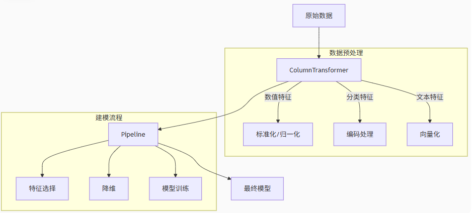
但是有没有发现，即使如此，看到这么多代码还是有有点晕，如果能用思维导图甚至是流程图的形式串起来代码逻辑就最好了，未来的内容我们来讲解流程图。
 

 

 通用模板：

from sklearn.compose import ColumnTransformer
from sklearn.pipeline import Pipeline
from sklearn.impute import SimpleImputer
from sklearn.preprocessing import StandardScaler, OneHotEncoder
from sklearn.feature_extraction.text import TfidfVectorizer
from sklearn.ensemble import RandomForestClassifier
from sklearn.feature_selection import SelectKBest
 
# 定义特征类型（需根据实际数据修改）
numerical_features = ['age', 'income']
categorical_features = ['gender', 'education']
text_features = ['product_review']
 
# 构建 ColumnTransformer
preprocessor = ColumnTransformer(
    transformers=[
        ('num', Pipeline(steps=[
            ('imputer', SimpleImputer(strategy='median')),
            ('scaler', StandardScaler())
        ]), numerical_features),
        ('cat', Pipeline(steps=[
            ('imputer', SimpleImputer(strategy='constant', fill_value='missing')),
            ('encoder', OneHotEncoder(handle_unknown='ignore'))
        ]), categorical_features),
        ('text', TfidfVectorizer(max_features=1000), text_features)
    ])
 
# 构建完整 Pipeline
full_pipeline = Pipeline(steps=[
    ('preprocessor', preprocessor),
    ('feature_selector', SelectKBest(k=50)),  # 可选特征选择
    ('classifier', RandomForestClassifier())
])

逻辑执行顺序

1.数据分类型处理：

1. 数值特征：缺失值填充，标准化
2. 分类特征：缺失值填充→独热编码
3. 文本特征：TF-DF向量化

2.特征级联：将处理后的各类特征水平拼接为统一矩阵

3.特征工程（可选） ：

1. 特征选择(如方差过滤、卡方检验)
2. 降维（如PCA、t-SNE)

4.模型训练：使用处理后的数据训练估计器 

 完整代码：

import pandas as pd
import numpy as np
import matplotlib.pyplot as plt
import seaborn as sns
import time
import warnings
from sklearn.pipeline import Pipeline
from sklearn.compose import ColumnTransformer
from sklearn.preprocessing import OrdinalEncoder, OneHotEncoder, StandardScaler
from sklearn.impute import SimpleImputer
from sklearn.ensemble import RandomForestClassifier
from sklearn.metrics import classification_report, confusion_matrix, accuracy_score, roc_curve, auc
from sklearn.model_selection import train_test_split
 
# 设置中文显示
plt.rcParams['font.sans-serif'] = ['SimHei', 'WenQuanYi Micro Hei', 'Heiti TC']
plt.rcParams['axes.unicode_minus'] = False
warnings.filterwarnings("ignore")
 
def load_and_preprocess_data(file_path):
    """加载数据并进行预处理"""
    # 加载数据
    data = pd.read_csv(file_path)
    print(f"数据加载完成，形状: {data.shape}")
    
    # 分离特征和目标变量
    X = data.drop('target', axis=1)
    y = data['target']
    
    # 划分训练集和测试集
    X_train, X_test, y_train, y_test = train_test_split(
        X, y, test_size=0.2, random_state=42, stratify=y
    )
    
    print("\n数据基本统计:")
    print(f"训练集大小: {X_train.shape}, 测试集大小: {X_test.shape}")
    print(f"目标变量分布: \n{y.value_counts(normalize=True)}")
    
    return X_train, X_test, y_train, y_test, X.columns
 
def build_preprocessing_pipeline(feature_names):
    """构建数据预处理Pipeline"""
    # 定义特征类型
    # 连续数值特征
    continuous_features = ['age', 'trestbps', 'chol', 'thalach', 'oldpeak']
    
    # 有序分类特征及其类别顺序
    ordinal_features = ['cp', 'restecg', 'slope', 'ca', 'thal']
    ordinal_categories = [
        [0, 1, 2, 3],       # cp: 胸痛类型
        [0, 1, 2],          # restecg: 静息心电图结果
        [0, 1, 2],          # slope: 运动峰值ST段斜率
        [0, 1, 2, 3, 4],    # ca: 主要血管染色数
        [0, 1, 2, 3]        # thal: 地中海贫血
    ]
    
    # 标称分类特征
    nominal_features = ['sex', 'fbs', 'exang']
    
    # 连续特征处理流程：填充缺失值并标准化
    continuous_transformer = Pipeline(steps=[
        ('imputer', SimpleImputer(strategy='mean')),
        ('scaler', StandardScaler())
    ])
    
    # 有序特征处理流程：填充缺失值并进行有序编码
    ordinal_transformer = Pipeline(steps=[
        ('imputer', SimpleImputer(strategy='most_frequent')),
        ('encoder', OrdinalEncoder(
            categories=ordinal_categories,
            handle_unknown='use_encoded_value',
            unknown_value=-1
        ))
    ])
    
    # 标称特征处理流程：填充缺失值并进行独热编码
    nominal_transformer = Pipeline(steps=[
        ('imputer', SimpleImputer(strategy='most_frequent')),
        ('onehot', OneHotEncoder(handle_unknown='ignore', sparse_output=False))
    ])
    
    # 构建ColumnTransformer
    preprocessor = ColumnTransformer(
        transformers=[
            ('continuous', continuous_transformer, continuous_features),
            ('ordinal', ordinal_transformer, ordinal_features),
            ('nominal', nominal_transformer, nominal_features)
        ],
        remainder='passthrough'
    )
    
    return preprocessor
 
def evaluate_model(pipeline, X_test, y_test):
    """评估模型性能并可视化结果"""
    # 预测
    y_pred = pipeline.predict(X_test)
    y_pred_proba = pipeline.predict_proba(X_test)[:, 1]
    
    # 计算准确率
    accuracy = accuracy_score(y_test, y_pred)
    print(f"\n模型准确率: {accuracy:.4f}")
    
    # 打印分类报告
    print("\n分类报告:")
    print(classification_report(y_test, y_pred))
    
    # 绘制混淆矩阵
    plt.figure(figsize=(8, 6))
    cm = confusion_matrix(y_test, y_pred)
    sns.heatmap(cm, annot=True, fmt='d', cmap='Blues')
    plt.xlabel('预测值')
    plt.ylabel('真实值')
    plt.title('混淆矩阵')
    plt.tight_layout()
    plt.savefig('confusion_matrix.png')
    
    # 绘制ROC曲线
    fpr, tpr, _ = roc_curve(y_test, y_pred_proba)
    roc_auc = auc(fpr, tpr)
    
    plt.figure(figsize=(8, 6))
    plt.plot(fpr, tpr, color='darkorange', lw=2, label=f'ROC曲线 (AUC = {roc_auc:.2f})')
    plt.plot([0, 1], [0, 1], color='navy', lw=2, linestyle='--')
    plt.xlim([0.0, 1.0])
    plt.ylim([0.0, 1.05])
    plt.xlabel('假阳性率')
    plt.ylabel('真阳性率')
    plt.title('ROC曲线')
    plt.legend(loc="lower right")
    plt.tight_layout()
    plt.savefig('roc_curve.png')
    
    return {
        'accuracy': accuracy,
        'classification_report': classification_report(y_test, y_pred),
        'confusion_matrix': cm,
        'roc_auc': roc_auc
    }
 
def main():
    # 数据加载与预处理
    X_train, X_test, y_train, y_test, feature_names = load_and_preprocess_data('D:\桌面\研究项目\打卡文件\python60-days-challenge-master\heart.csv')
    
    # 构建预处理Pipeline
    preprocessor = build_preprocessing_pipeline(feature_names)
    
    # 构建完整Pipeline
    pipeline = Pipeline(steps=[
        ('preprocessor', preprocessor),
        ('classifier', RandomForestClassifier(random_state=42))
    ])
    
    # 训练模型
    print("\n开始训练模型...")
    start_time = time.time()
    pipeline.fit(X_train, y_train)
    end_time = time.time()
    
    print(f"模型训练完成，耗时: {end_time - start_time:.4f} 秒")
    
    # 评估模型
    metrics = evaluate_model(pipeline, X_test, y_test)
    
    # 特征重要性分析
    if hasattr(pipeline.named_steps['classifier'], 'feature_importances_'):
        try:
            # 获取特征重要性
            feature_importance = pipeline.named_steps['classifier'].feature_importances_
            
            # 获取预处理后的特征名称
            preprocessor = pipeline.named_steps['preprocessor']
            ohe = preprocessor.named_transformers_['nominal'].named_steps['onehot']
            feature_names = (
                preprocessor.transformers_[0][2] +  # 连续特征
                preprocessor.transformers_[1][2] +  # 有序特征
                ohe.get_feature_names_out(preprocessor.transformers_[2][2]).tolist()  # 标称特征
            )
            
            # 绘制特征重要性图
            plt.figure(figsize=(10, 6))
            plt.barh(feature_names, feature_importance)
            plt.xlabel('特征重要性')
            plt.ylabel('特征名称')
            plt.title('随机森林特征重要性')
            plt.tight_layout()
            plt.savefig('feature_importance.png')
            
            print("\n特征重要性分析已保存为 feature_importance.png")
        except Exception as e:
            print(f"无法绘制特征重要性图: {e}")
    
    print("\n模型训练和评估完成！")
    print("结果已保存为 confusion_matrix.png, roc_curve.png 和 feature_importance.png")
 
if __name__ == "__main__":
    main()

 @浙大疏锦行