信号与系统实验一 信号在MATLAB中的表示

• 实验目的

1. 掌握运用MATLAB表示常用连续和离散时间信号的方法。
2. 观察并熟悉这些信号的波形和特性。

• 实验设备

1. 计算机。
2. MATLAB软件。

• 实验内容

1. 实验教程p8练习一，1。
2. 绘出下列信号波形图：
   1. 1. 教材 p39, 1-4(2)；
      2. 教材 p39, 1-4(3)。
3. 用下列函数各画一图，参数自定。

sinc, rectpuls, square, tripuls, sawtooth

四、实验步骤

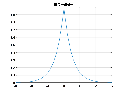
1.信号一：y1（t）=e-2|t|

源程序：

A=1;

a=-2;

t=-3:0.01:3;

yt=A*exp(a*abs(t));  %abs（t）在MATLAB中表示t的绝对值。  

plot(t,yt),grid on   %MATLAB函数中连续时间信号绘图用plot函数。

axis([-3,3,0,1])

title('练习一函数一')

图像：

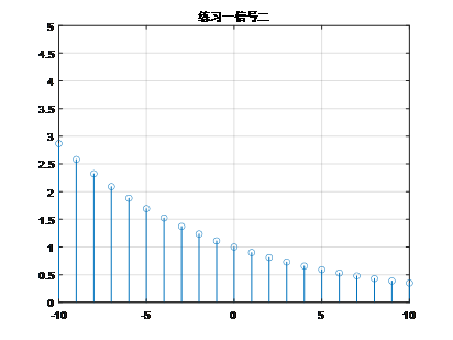
2.信号二：y2（n）=（0.9）n（-10≤n≤10）

源程序：

          a=0.9;

n=-10:10;

yn=a.^n;  %在MATLAB中a的n次方用a.^n表示。

stem(n,yn);  %离散时间信号用绘图用stem函数。

grid on  

axis([-10,10,0,5])

title('练习一信号二')

图像：

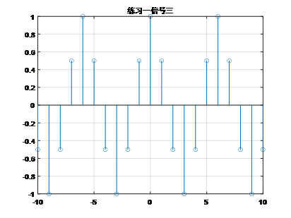
3.信号三：y3（n）=eiΠn/3（-10≤n≤10）的实部。

 源程序：

          n=-10:10;

yn=real(exp(i*pi*n/3));  %在MATLAB中real函数表示取实部。

stem(n,yn),grid on

axis([-10,10,-1,1])

title('练习一信号三')

图像：

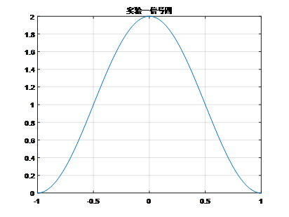
4.信号四：x1（t）=（1+cosΠt） （-1＜t＜1）

     源程序：

t=-1:0.01:1;

w=pi;

xt=1+cos(w*t);  

plot(t,xt),grid on

axis([-1,1,0,2])

title('实验一信号四')

图像：

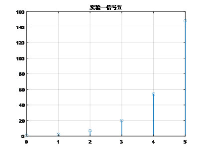
5.信号五：x2[n]=en    （0≤n＜5）

源程序：

n=0:5;

xn=floor(exp(n));  %MATLAB中取整用floor函数。

stem(n,xn),grid on

axis([0,5,0,160])

title('实验一信号五')

      图像：

           

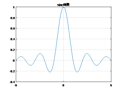
6.sinc函数：f1（t）=sinc（t）

  源程序：

        t=-5:0.01:5;

ft=sinc(t);

plot(t,ft),grid on

axis([-5,5,-0.4,1])

title('sinc函数')

图像：

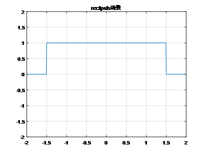
7.rectpuls函数：f1（t）=rectpuls（t）

源程序：

      t=-2:0.01:2;

ft=rectpuls(t,3);

plot(t,ft),grid on

axis([-2,2,-2,2])

title('rectpuls函数')

图像：

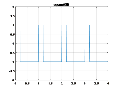
1. square函数：f（t）=square（t）

      源程序：

      t=0:0.01:4;

ft=square(2*pi*t,20);  %MATLAB中square函数表示周期性矩形波信号

plot(t,ft),grid on

axis([0,4,-2,2])

title('square函数')

         图像：

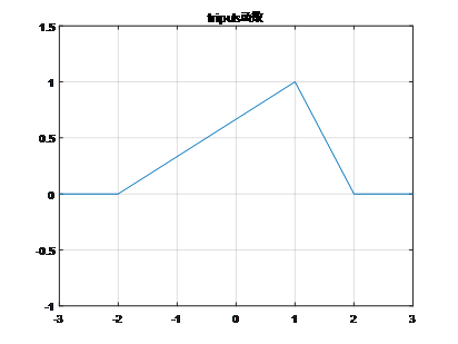
1. tripuls函数：f（t）=tripuls（t）

源程序：

t=-3:0.001:3;

ft=tripuls(t,4,0.5);

plot(t,ft),grid on

axis([-3,3,-1,1.5])

title('tripuls函数')

图像：

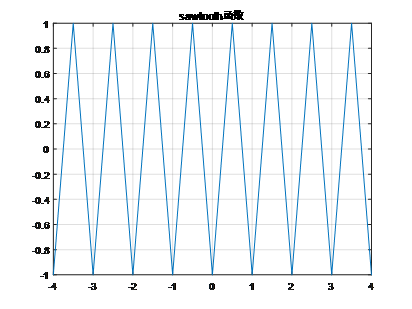
1. sawtooth函数：f（t）=sawtooth（t）

     源程序：

t=-4:0.001:4;

ft=sawtooth(2*pi*t,0.5)

plot(t,ft),grid on

axis([-4,4,-1,1])

title('sawtooth函数')

      图像：

五、实验总结

  1.注意MATLAB中连续时间信号与离散时间信号绘图所用函数不同，前者用plot函数，后者用stem函数。

2. 使用MATLAB绘图时，用axis函数规定横纵坐标的取值范围，注意取值适当，使其显示出图像的全部信息。

3.实验时需牢记各个函数的调用格式，以及各个设值所代表的含义，不可盲目使用。

4.遇到不理解的代码或函数，可在命令行窗口输入“help 不理解的代码”即可出现其解释与用法；在命令行窗口输入“clc”+回车可清除命令行窗口的内容。