【深度学习入门】NNDL学习笔记（二）

 

Chapter2 How the backpropagation algorithm works?

反向传播 Backpropagation: a fast algorithm for computing gradients.

Warm up: a fast matrix-based approach to computing the output from a neural network

                                                      

weighted input: 

elementwise multiplication: 

The two assumptions we need about the cost function

1. The cost function can be written as an average over cost functions Cx for individual training examples, x.

2. The cost can be written as a function of the outputs from the neural network 

The four fundamental equations behind backpropagation

The error  in the jth neuron in the lth layer: 

For all σ(.)： 

Equation1: the error in the output layer 

---

                                                                     ,

                                                            matrix form: 

---

It is easily computed: 

因为, 计算出z 就可计算出 ；

If we're using the quadratic cost function then ,   

matrix form 

Equation2: the error  in terms of the next layer, 

---

                                                                 ,

                                                                      

---

Equation3: An equation for the rate of change of the cost with respect to any bias in the network.

---

                                                                 

---

Equation4: An equation for the rate of change of the cost with respect to any weight in the network

---

                                                          ,     

---

A weight or bias in the final layer will learn slowly if the output neuron is either low activation (≈0) or high activation (≈1). 

If the input neuron is low-activation, or if the output neuron has saturated, weights and biases will learn very slowly.

The backpropagation algorithm

Exercise

1.Suppose we modify a single neuron in a feedforward network so that the output from the neuron is given by f(∑jwjxj+b). How should we modify the backpropagation algorithm in this case?

For BP1 & BP2 just exchange σ for f while BP3 & BP4 will not change.

2.Linear: Suppose we replace the usual non-linear σ function with σ(z)=z throughout the network. Rewrite the backpropagation algorithm for this case.

Change every σ to f(z) = x.

The code for backpropagation

For a mini-batch of size m:

Fully matrix-based approach： It's possible to modify the backpropagation algorithm so that it computes the gradients for all training examples in a mini-batch simultaneously，taking full advantage of modern libraries for linear algebra

The big picture

                                                                     

 

This suggests that a possible approach to computing ∂C/∂wljk is to carefully track how a small change in wljk propagates to cause a small change in C.

                                                                    

For a single neuron in the next layer:

                                                                   

Imagine a path from w to C:

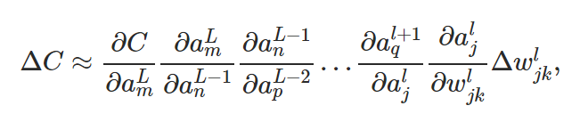
There are many paths from w to C:

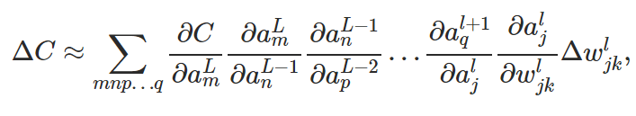
What the equation tells us is that every edge between two neurons in the network is associated with a rate factor which is just the partial derivative of one neuron's activation with respect to the other neuron's activation.