7月20日数据科学库学习笔记——pandas 字符串离散化、数据合并、分组聚合、复合索引

---

前言

本文为7月20日数据科学库学习笔记，分为四个章节：

• 字符串离散化；
• 数据合并：.join()、.merge()；
• 数据分组聚合；
• 数据的复合索引：Series 复合索引、DataFrame 复合索引。

---

一、字符串离散化

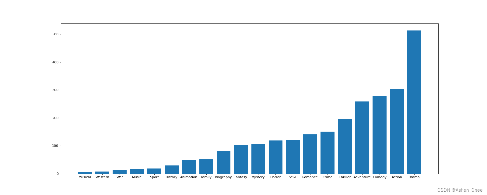
• 示例：对于之前的电影数据，统计电影的分类（Genre）情况——构造一个全为0的数组，列名为分类，若某一条数据中分类出现过，就让0变为1。

import numpy as np
import pandas as pd
from matplotlib import pyplot as plt
import string

file_path = './IMDB-Movie-Data.csv'

df = pd.read_csv(file_path)

# 统计分类的列表
temp_list = df["Genre"].str.split(',').tolist()  # 列表嵌套列表

# 去重
genre_list = list(set([i for j in temp_list for i in j]))

#构造全为 0 的列表
zeros_df = pd.DataFrame(np.zeros((df.shape[0], len(genre_list))), columns=genre_list)
# print(zeros_df)

# 给每个电影出现分类的位置赋值1
for i in range(df.shape[0]):
    # zeros_df.loc[0, ["Sci-fi", "Musical"]] = 1
    zeros_df.loc[i, temp_list[i]] = 1

# print(zeros_df.head(3))

# 统计每个分类的电影的数量和
genre_count = zeros_df.sum(axis=0)
print(genre_count)

# 排序
genre_count = genre_count.sort_values()
_x = genre_count.index
_y = genre_count.values

# 画图
plt.figure(figsize=(20, 8), dpi=80)
plt.bar(range(len(_x)), _y)
plt.xticks(range(len(_x)), _x)

plt.show()

>>> Comedy       279.0
    Mystery      106.0
    Family        51.0
    Drama        513.0
    Romance      141.0
    Sport         18.0
    Sci-Fi       120.0
    Horror       119.0
    Animation     49.0
    Western        7.0
    Musical        5.0
    History       29.0
    Music         16.0
    Action       303.0
    Biography     81.0
    Fantasy      101.0
    Crime        150.0
    Thriller     195.0
    War           13.0
    Adventure    259.0

---

二、数据合并

1、.join()

把行索引相同的数据合并到一起：

t1
>>>      0    1    2    3
    A  1.0  1.0  1.0  1.0
    B  1.0  1.0  1.0  1.0
    C  1.0  1.0  1.0  1.0

t2
>>>      V    W    X    Y    Z
    A  0.0  0.0  0.0  0.0  0.0
    B  0.0  0.0  0.0  0.0  0.0

t1.join(t2)
>>>      0    1    2    3    V    W    X    Y    Z
    A  1.0  1.0  1.0  1.0  0.0  0.0  0.0  0.0  0.0
    B  1.0  1.0  1.0  1.0  0.0  0.0  0.0  0.0  0.0
    C  1.0  1.0  1.0  1.0  NaN  NaN  NaN  NaN  NaN

2、.merge()

按照指定的列把数据按一定的方式合并到一起。

(1)、inner 默认的合并方式——交集

t1
>>>      M    N  O    P
    A  1.0  1.0  a  1.0
    B  1.0  1.0  b  1.0
    C  1.0  1.0  c  1.0

t2
>>>      V    W  X    Y    Z
    A  0.0  0.0  c  0.0  0.0
    B  0.0  0.0  d  0.0  0.0

t1.merge(t2, left_on="O", right_on='X')
     M    N  O    P    V    W  X    Y    Z
0  1.0  1.0  c  1.0  0.0  0.0  c  0.0  0.0

(2)、how=“outer”——并集

t1
>>>      M    N  O    P
    A  1.0  1.0  a  1.0
    B  1.0  1.0  b  1.0
    C  1.0  1.0  c  1.0

t2
>>>      V    W  X    Y    Z
    A  0.0  0.0  c  0.0  0.0
    B  0.0  0.0  d  0.0  0.0

t1.merge(t2, left_on='O', right_on="X", how='outer')
>>>      M    N    O    P    V    W    X    Y    Z
    0  1.0  1.0    a  1.0  NaN  NaN  NaN  NaN  NaN
    1  1.0  1.0    b  1.0  NaN  NaN  NaN  NaN  NaN
    2  1.0  1.0    c  1.0  0.0  0.0    c  0.0  0.0
    3  NaN  NaN  NaN  NaN  0.0  0.0    d  0.0  0.0

(3)、how=“left”|“right”——左边或右边为准

t1
>>>      M    N  O    P
    A  1.0  1.0  a  1.0
    B  1.0  1.0  b  1.0
    C  1.0  1.0  c  1.0

t2
>>>      V    W  X    Y    Z
    A  0.0  0.0  c  0.0  0.0
    B  0.0  0.0  d  0.0  0.0

t1.merge(t2, left_on='O', right_on="X", how='left')
>>>      M    N  O    P    V    W    X    Y    Z
    0  1.0  1.0  a  1.0  NaN  NaN  NaN  NaN  NaN
    1  1.0  1.0  b  1.0  NaN  NaN  NaN  NaN  NaN
    2  1.0  1.0  c  1.0  0.0  0.0    c  0.0  0.0

t1.merge(t2, left_on='O', right_on="X", how='right')
>>>      M    N    O    P    V    W  X    Y    Z
    0  1.0  1.0    c  1.0  0.0  0.0  c  0.0  0.0
    1  NaN  NaN  NaN  NaN  0.0  0.0  d  0.0  0.0

---

三、数据分组聚合

用法：grouped = df.groupby(by="columns_name")

• grouped 是一个 DataFrameGroupBy 对象，可迭代；
• grouped 中的每一个元素是一个元组。

示例：统计美国和中国的星巴克的数量：

file_path = './starbucks_store_worldwide.csv'

df = pd.read_csv(file_path)
# print(df.head(1))
# print(df.info())

grouped = df.groupby(by="Country")  # DataFrameGroupBy 对象

# 调用聚合方法
country_count = grouped["Brand"].count()
print(country_count["US"])
print(country_count["CN"])

>>> 13608
>>> 2734

• 其他方法：
  

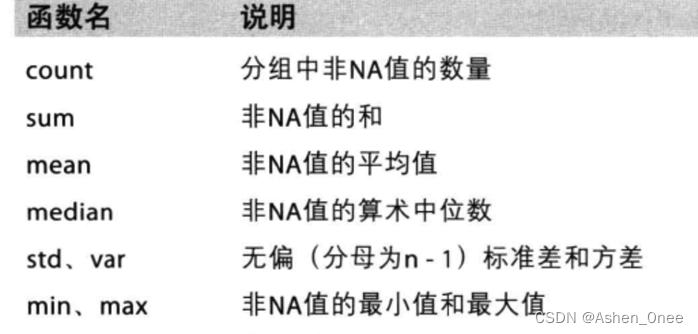
• 对国家和省份进行分组统计：
  grouped = df.groupby(by=[df["Country"], df["State/Province"]])

• 获取分组之后的某一部分数据：
  df.groupby(by=["Country", "State/Province"])["Country"].count()

• 对某几列数据进行分组：
  df["Country"].groupby(by=[df["Country"], df["State/Province"]]).count()

---

四、数据的索引&复合索引

1、Series 复合索引

• 获取index：df.index；
• 指定index ：df.index = [‘x’,‘y’]；
• 重新设置index : df.reindex(list(“abcedf”))；
• 指定某一列作为index：df.set_index(“Country”,drop=False)；
• 返回index的唯一值；
• df.set_index(“Country”).index.unique()。

设置两个索引的结果：

a
>>>    a  b    c  d
    0  0  7  one  h
    1  1  6  one  j
    2  2  5  one  k
    3  3  4  two  l

X = a.set_index(["c", "d"])["a"]
X
>>>      c    d
    one  h    0
         j    1
         k    2
    two  l    3
         m    4
         n    5
         o    6

X["one", "h"]
>>> 0

取索引 h 对应值：
X.swaplevel()，level 相当于复合索引的里外层，交换了 level后，里外交换

X.swaplevel()["h"]
>>> c
    one    0

2、DataFrame 复合索引

• 转换成 DataFrame 格式：

a
>>>    a  b    c  d
    0  0  7  one  h
    1  1  6  one  j
    2  2  5  one  k
    3  3  4  two  l

x = a.set_index(["c", "d"])[["a"]]
x
           a
>>> c   d   
    one h  0
        j  1
        k  2
    two l  3
        m  4
        n  5
        o  6

• 取索引的值：

x
           a
>>> c   d   
    one h  0
        j  1
        k  2
    two l  3
        m  4
        n  5
        o  6

x.loc["one"]
>>>    a
    d   
    h  0
    j  1
    k  2
    
x.loc["one"].loc["h"]
>>> a    0

x.swaplevel().loc["h"]
>>>      a
    c     
    one  0

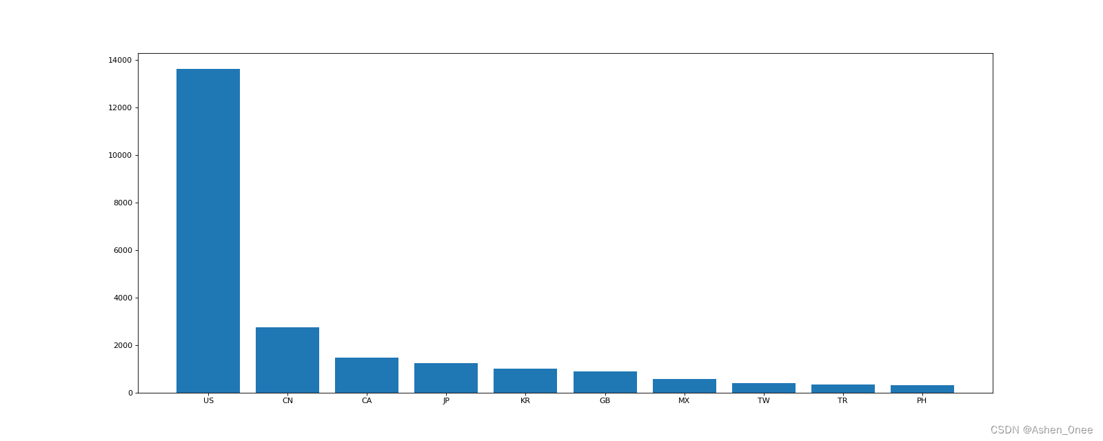
示例：呈现店铺总数排名前10的国家：

import pandas as pd
import numpy as np
from matplotlib import pyplot as plt

file_path = './starbucks_store_worldwide.csv'

df = pd.read_csv(file_path)

# 呈现店铺总数排名前10的国家

# 准备数据
data1 = df.groupby(by="Country").count()["Brand"].sort_values(ascending=False)[:10]

_x = data1.index
_y = data1.values

# 画图
plt.figure(figsize=(20, 8), dpi=80)

plt.bar(range(len(_x)), _y)
plt.xticks(range(len(_x)), _x)

plt.show()

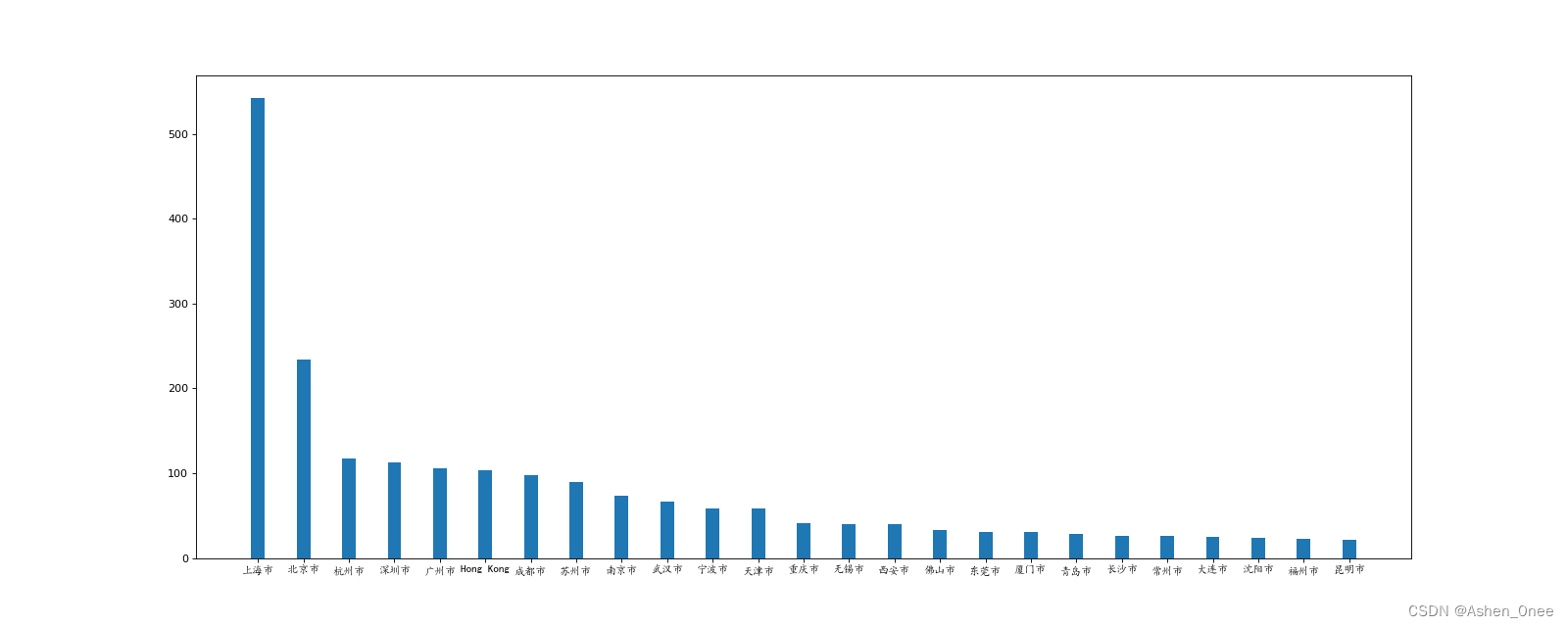
示例：呈现中国每个城市的店铺数量：

import pandas as pd
import numpy as np
from matplotlib import pyplot as plt
from matplotlib import font_manager

my_font = font_manager.FontProperties(fname=r'C:\Windows\Fonts\SIMKAI.ttf')

file_path = './starbucks_store_worldwide.csv'

df = pd.read_csv(file_path)
df = df[df["Country"]=="CN"]
print(df.head(1))

# 呈现中国每个城市的店铺数量

# 准备数据
data1 = df.groupby(by="City").count()["Brand"].sort_values(ascending=False)[:25]

_x = data1.index
_y = data1.values

# 画图
plt.figure(figsize=(20, 8), dpi=80)

plt.bar(range(len(_x)), _y, width=0.3)
plt.xticks(range(len(_x)), _x, fontproperties=my_font)

plt.show()

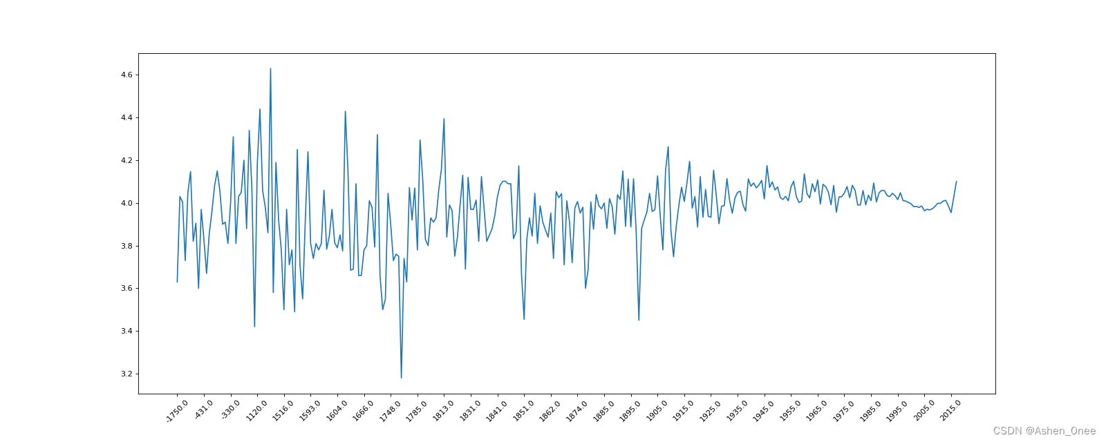
示例：有全球排名靠前的10000本书的数据，统计不同年份书的平均评分情况：

import pandas as pd
from matplotlib import pyplot as plt

file_path = './books.csv'

df = pd.read_csv(file_path)
# print(df.info())

# 不同年份的书平均评分情况
# 去除 original_publication_year中 nan 的行
data1 = df[pd.notnull(df["original_publication_year"])]

grouped = data1["average_rating"].groupby(by=data1["original_publication_year"]).mean()

print(grouped)

_x = grouped.index
_y = grouped.values

plt.figure(figsize=(20, 8), dpi=80)
plt.plot(range(len(_x)), _y)
plt.xticks(list(range(len(_x)))[::10], _x[::10], rotation=45)

plt.show()

---