9月16日计算机视觉基础学习笔记——认识机器视觉

---

前言

本文为9月16日计算机视觉基础学习笔记——认识机器视觉，分为四个章节：

• Week 1 homework；
• 从图像处理到计算机视觉；
• 计算机视觉的两个步骤；
• 图像描述子。

---

一、Week 1 homework

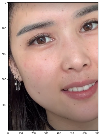
1、基本操作

import cv2 as cv
import matplotlib.pyplot as plt
import numpy as np

img = cv.imread("week1_homework.png")
img_RGB = cv.cvtColor(img, cv.COLOR_BGR2RGB)

plt.figure(figsize=(10, 10))
plt.imshow(img_RGB)
plt.show()

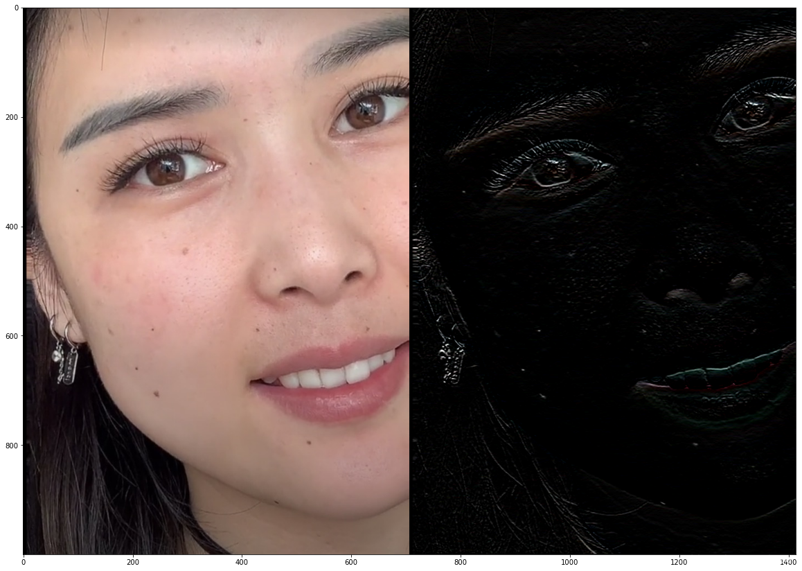
2、滤波

# 滤波
# 边缘提取
kernel = np.ones((3, 3), np.float32) / 9   # 平均滤波

# X 方向梯度
# kernel[0, :] = [-1, 0, 1]
# kernel[1, :] = [-1, 0, 1]
# kernel[2, :] = [-1, 0, 1]

# Y 方向梯度
kernel[0, :] = [-1, -1, -1]
kernel[1, :] = [0, 0, 0]
kernel[2, :] = [1, 1, 1]


print(kernel)
>>> [[-1. -1. -1.]
     [ 0.  0.  0.]
     [ 1.  1.  1.]]

print(img_RGB.shape)
>>> (1000, 707, 3)

result = cv.filter2D(img_RGB, -1, kernel)
print(result.shape)
>>> (1000, 707, 3)
print(result[0, 0])
>>> [0 0 0]

plt.figure(figsize=(20, 20))
plt.imshow(cv.hconcat([img_RGB, result])) # 水平拼接
plt.show()

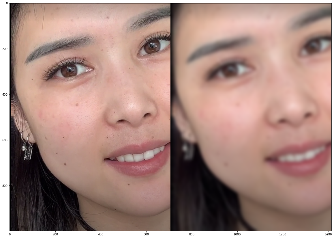
• 更大滤波核 & 更多次滤波：

# 更大滤波核 & 更多次滤波
kernel = np.ones((15, 15), np.float32) / (15 * 15)

img1 = cv.filter2D(img_RGB, -1, kernel)
result = cv.filter2D(img1, -1, kernel)

# 显示滤波前后对比
plt.figure(figsize=(20, 20))
plt.imshow(cv.hconcat([img_RGB, result]))
plt.show()

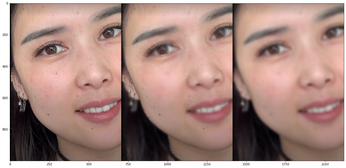
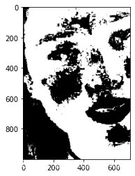
• 只对肤色区域滤波：

result_show = result.copy()
# 肤色检测
hsv = cv.cvtColor(img, cv.COLOR_BGR2HSV)
(_h, _s, _v) = cv.split(hsv) # 图像分割，分别获取 h，s，v通道分量图像
print(_h.shape)
>>> (1000, 707)

skin3 = np.zeros(_h.shape, dtype = np.uint8)  # 根据源图像的大小创建一个全0的矩阵,用于保存图像数据
(x, y) = _h.shape  # 获取图像数据的长和宽

# 遍历图像。判断 HSV 通道的数值，若在指定范围中，则设置像素点为 255， 否则设为 0
for i in range(0, x):
    for j in range(0, y):
        if (5 < _h[i][j] < 70) and (_s[i][j] > 18) and (50 < _v[i][j] < 255):
            skin3[i][j] = 1.0
            result_show[i][j] = img_RGB[i][j] * skin3[i][j]
        else:
            skin3[i][j] = 0.0
        
# result_show_RGB = cv.cvtColor(result_show, cv.COLOR_BGR2RGB)

plt.figure(figsize=(20, 20))
plt.imshow(cv.hconcat([img_RGB, result_show_RGB, result]))
plt.show()

skin3 = cv.cvtColor(skin3, cv.COLOR_BGR2RGB)
plt.imshow(skin3)
plt.show()

---

二、从图像处理到计算机视觉

import cv2 as cv
import matplotlib.pyplot as plt
import sys
import os

def BGRtoRGB(img):
    return cv.cvtColor(img, cv.COLOR_BGR2RGB)

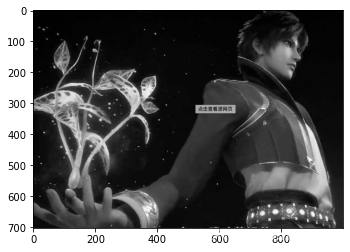
img = cv.imread("tangsan.jpg")
dog = cv.imread("dog.png")

gray = cv.cvtColor(img, cv.COLOR_BGR2GRAY)
dog_gray = cv.cvtColor(dog, cv.COLOR_BGR2GRAY)
print(dog.shape)
>>> (852, 590, 3)

plt.figure(figsize=(11, 11))
plt.imshow(BGRtoRGB(img))
plt.show()

plt.imshow(gray, cmap="gray")
plt.show()

1、反色变换

reverse_c = img.copy()
rows = img.shape[0]
cols = img.shape[1]
depths = img.shape[2]

for i in range(rows):
    for j in range(cols):
        for d in range(depths):
            reverse_c[i][j][d] = 255 - reverse_c[i][j][d]
            
plt.imshow(BGRtoRGB(cv.hconcat([img, reverse_c])))
plt.show()

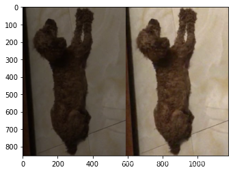
2、Gamma 变换

gamma_c = dog.copy()
rows = dog.shape[0]
cols = dog.shape[1]
depths = dog.shape[2]

for i in range(rows):
    for j in range(cols):
        for d in range(depths):
            gamma_c[i][j][d] = 3 * pow(gamma_c[i][j][d], 0.9)
            
plt.imshow(BGRtoRGB(cv.hconcat([dog, gamma_c])))
plt.show()       

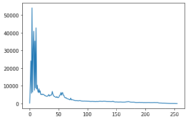
3、直方图 & 直方图均衡化

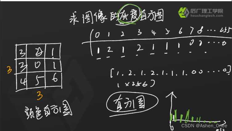
• 计算直方图：

import numpy as np

hist = np.zeros(256)

rows = img.shape[0]
cols = img.shape[1]

for i in range(rows):
    for j in range(cols):
        tmp = gray[i][j]
        hist[tmp] = hist[tmp] + 1

plt.plot(hist)
plt.show()

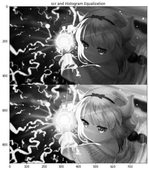
• 直方图均衡化：

trans = hist / (rows * cols) * 255
for i in range(1, len(trans)):
    trans[i] = trans[i-1] + trans[i]

print(int(trans[0]))
print(trans.shape)
>>> 0
>>> (256,)

gray_h = gray.copy()
for i in range(rows):
    for j in range(cols):
        gray_h[i][j] = int(trans[gray[i][j]])

plt.figure(figsize=(10,10))
plt.imshow(cv.vconcat([gray,gray_h]),cmap='gray')
plt.title("scr and Histogram Equalization")
plt.show()

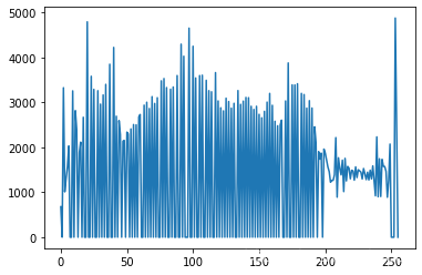
hist_h = np.zeros(256)
for i in range(rows):
    for j in range(cols):
        tmp = gray_h[i][j]
        hist_h[tmp] = hist_h[tmp] + 1
        
plt.plot(hist_h)
plt.show()

---

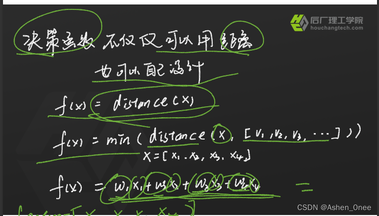
三、计算机视觉的两个步骤

1、提取特征 feature

2、决策函数

---

四、图像描述子

1、HOG（Histogram of Oriented Gradient）

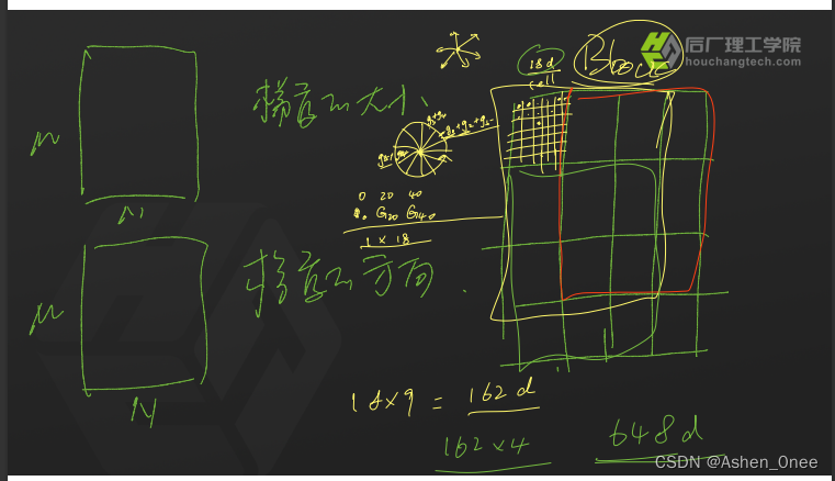
• 步骤：
  1. 灰度化 + Gamma 变换 / 直方图均衡化；
  2. 计算每个像素的梯度（大小 + 方向）：
     $$\begin{gathered} \frac{DG(x,y)}{Dx}=G(x+1,y)-G(x-1,y) \\ \frac{DG(x,y)}{Dy}=G(x,y+)-G(x,y-1) \end{gathered}$$

     • 相当于卷积：
       $$\left[\begin{array}{ccc}0& -1& 0\\ -1& 0& 1\\ 0& 1& 0\end{array}\right]=\left[\begin{array}{c}-1\\ 0\\ 1\end{array}\right]\left[\begin{array}{ccc}-1& 0& 1\end{array}\right]$$

     • 得到两张图：

       • 梯度的大小：$\sqrt{D_x^2+D_y^2}$；
       • 梯度的方向：$arctan\frac{D_y}{D_x}$.
  3. 将图像分成小 cells（6×6）
  4. 统计每个 cell 的梯度直方图，每个 cell 一个结果（Description 描述子——18维）；
  5. 将每 3×3 个 cell 组成一个 block，每个 cell 的结果串起来，得到 block 的结果（Description——162维），然后归一化，即我们需要的结果。

2、LBP（Local Binary Pattern）

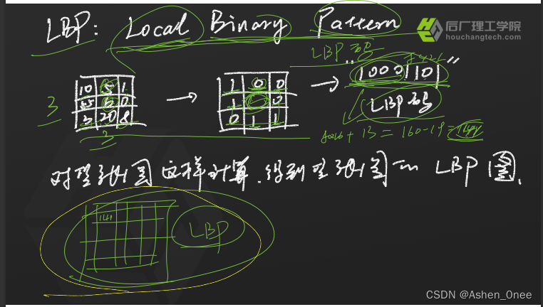
局部二值模式。

• 步骤：
  1. 将图像分成 16×16 的cell；
  2. 对 cell 中的每个像素计算其对应的 LBP 值；
  3. 计算每个 cell 的直方图，然后归一化；
  4. 将每个 cell 的直方图连起来，就得到这张图的描述子。

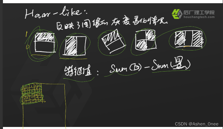
3、Haar-like

反映图像的灰度变化情况。

---