VARIATIONAL IMAGE COMPRESSION WITH A SCALE HYPERPRIOR

VARIATIONAL IMAGE COMPRESSION WITH A SCALE HYPERPRIOR

ABSTRACT

We describe an end-to-end trainable model for image compression based on variational autoencoders.The model incorporates a hyperprior to effectively capture spatial dependencies in the latent representation.This hyperprior relates to side information, a concept universal to virtually all modern image codecs, but largely unexplored in image compression using artificial neural networks (ANNs).Unlike existing autoencoder compression methods, our model trains a complex prior jointly with the underlying autoencoder. We demonstrate that this model leads to state-of-the-art image compression when measuring visual quality using the popular MS-SSIM index, and yields rate–distortion performance surpassing pub- lished ANN-based methods when evaluated using a more traditional metric based on squared error (PSNR).Furthermore, we provide a qualitative comparison of models trained for different distortion metrics.

我们描述了一种基于变分自动编码器的端到端可训练图像压缩模型。该模型结合了超先验来有效捕获潜在表示中的空间依赖性。这个超先验与辅助信息有关，这是一个几乎所有现代图像编解码器都通用的概念，但在使用人工神经网络 (ANN) 的图像压缩中很大程度上尚未得到探索。与现有的自动编码器压缩方法不同，我们的模型与底层自动编码器联合训练复杂的先验。我们证明，当使用流行的 MS-SSIM 指数测量视觉质量时，该模型可以实现最先进的图像压缩，并且当使用更传统的基于度量的评估时，其率失真性能超过已发布的基于 ANN 的方法。平方误差 (PSNR)。此外，我们还对针对不同失真指标训练的模型进行了定性比较。

1 INTRODUCTION

Recent machine learning methods for lossy image compression have generated significant interest in both the machine learning and image processing communities (e.g., Ballé et al., 2017; Theis et al., 2017; Toderici et al., 2017; Rippel and Bourdev, 2017).Like all lossy compression methods, they operate on a simple principle: an image, typically modeled as a vector of pixel intensities x, is quantized, reducing the amount of information required to store or transmit it, but introducing error at the same time.Typically, it is not the pixel intensitites that are quantized directly.Rather, an alternative (latent) representation of the image is found, a vector in some other space y, and quanti- zation takes place in this representation, yielding a discrete-valued vector ˆy.Because it is discrete, it can be losslessly compressed using entropy coding methods, such as arithmetic coding (Rissanen and Langdon, 1981), to create a bitstream which is sent over the channel. Entropy coding relies on a prior probability model of the quantized representation, which is known to both encoder and decoder (the entropy model).

最近用于有损图像压缩的机器学习方法引起了机器学习和图像处理社区的极大兴趣（例如，Ballé 等人，2017 年；Theis 等人，2017 年；Toderici 等人，2017 年；Rippel 和 Bourdev，2017 年） ）。与所有有损压缩方法一样，它们的工作原理很简单：图像（通常建模为像素强度 x 的向量）被量化，减少了存储或传输图像所需的信息量，但同时引入了误差。通常，像素强度不是直接量化的。相反，找到图像的替代（潜在）表示，即其他空间 y 中的向量，并在该表示中进行量化，产生离散值向量 ^y。因为它是离散的，所以可以使用熵编码方法（例如算术编码（Rissanen 和 Langdon，1981））对其进行无损压缩，以创建通过通道发送的比特流。熵编码依赖于量化表示的先验概率模型，编码器和解码器都知道该模型（熵模型）。

In the class of ANN-based methods for image compression mentioned above, the entropy model used to compress the latent representation is typically represented as a joint, or even fully factorized, distribution pˆy (ˆy).Note that we need to distinguish between the actual marginal distribution of the latent representation m(ˆy), and the entropy model pˆy (ˆy).While the entropy model is typically as- sumed to have some parametric form, with parameters fitted to the data, the marginal is an unknown distribution arising from both the distribution of images that are encoded, and the method which is used to infer the alternative representation y.The smallest average code length an encoder–decoder pair can achieve, using pˆy as their shared entropy model, is given by the Shannon cross entropy between the two distributions:

在上述基于 ANN 的图像压缩方法中，用于压缩潜在表示的熵模型通常表示为联合分布，甚至完全分解的分布 pˆy (ˆy)。请注意，我们需要区分潜在表示 m(ˆy) 的实际边缘分布和熵模型 pˆy (ˆy)。虽然熵模型通常被假设为具有某种参数形式，并且参数适合数据，但边际是由编码图像的分布以及用于推断替代表示的方法产生的未知分布y。使用 pˆy 作为共享熵模型，编码器-解码器对可以实现的最小平均代码长度由两个分布之间的香农交叉熵给出：

(1)

Note that this entropy is minimized if the model distribution is identical to the marginal.This implies that, for instance, using a fully factorized entropy model, when statistical dependencies exist in the actual distribution of the latent representation, will lead to suboptimal compression performance.

请注意，如果模型分布与边际分布相同，则该熵会最小化。这意味着，例如，使用完全分解的熵模型，当潜在表示的实际分布中存在统计依赖性时，将导致次优的压缩性能。

One way conventional compression methods increase their compression performance is by transmitting side information: additional bits of information sent from the encoder to the decoder, which signal modifications to the entropy model intended to reduce the mismatch.This is feasible because the marginal for a particular image typically varies significantly from the marginal for the ensemble of images the compression model was designed for.In this scheme, the hope is that the amount of side information sent is smaller, on average, than the reduction of code length achieved in eq.(1) by matching pˆy more closely to the marginal for a particular image.For instance, JPEG (1992) models images as independent fixed-size blocks of 8 × 8 pixels.However, some image structure, such as large homogeneous regions, can be more efficiently represented by considering larger blocks at a time.For this reason, more recent methods such as HEVC (2013) partition an image into variable- size blocks, convey the partition structure to the decoder as side information, and then compress the blockrepresentations using that partitioning.That is, the entropy model for JPEG is always factorized into groups of 64 elements, whereas the factorization is variable for HEVC.The HEVC decoder needs to decode the side information first, so that it can use the correct entropy modelto decode the block representations.Since the encoder is free to select a partitioning that optimizes the entropy model for each image, this scheme can be used to achieve more efficient compression.

传统压缩方法提高其压缩性能的一种方法是传输辅助信息：从编码器发送到解码器的附加信息位，这些信息表示对熵模型的修改旨在减少不匹配。这是可行的，因为特定图像通常与压缩模型设计的图像集合的边缘有显着差异。在该方案中，希望发送的辅助信息量平均小于等式(1) 中实现的代码长度的减少。 通过将 pˆy 与特定图像的边缘更紧密地匹配。例如，JPEG (1992) 将图像建模为 8 × 8 像素的独立固定大小块。然而，某些图像结构（例如大的均匀区域）可以通过一次考虑较大的块可以更有效地表示。因此，最近的方法如 HEVC (2013) 将图像划分为可变大小的块，将分区结构作为辅助信息传递给解码器，然后压缩块也就是说，JPEG 的熵模型始终分解为 64 个元素的组，而 HEVC 的分解是可变的。HEVC 解码器需要首先解码辅助信息，以便可以使用正确的熵模型解码块表示。由于编码器可以自由选择优化每个图像的熵模型的分区，因此该方案可用于实现更有效的压缩。

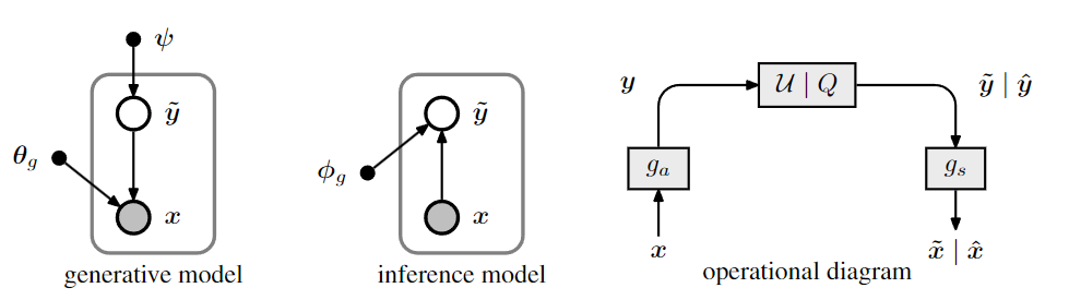
Figure 1: Left: representation of a transform coding model as a generative Bayesian model, and a
corresponding variational inference model. Nodes represent random variables or parameters, and
arrows indicate conditional dependence between them. Right: diagram showing the operational
structure of the compression model. Arrows indicate the flow of data, and boxes represent transfor-
mations of the data. Boxes labeled U | Q represent either addition of uniform noise applied during
training (producing vectors labeled with a tilde), or quantization and arithmetic coding/decoding
during testing (producing vectors labeled with a hat)

图 1：左：将变换编码模型表示为生成贝叶斯模型，以及相应的变分推理模型。节点表示随机变量或参数，箭头表示它们之间的条件依赖关系。右图：显示压缩模型的运行结构的图表。箭头表示数据流，方框表示数据的转换。标有 U | 的盒子Q 表示在训练期间添加均匀噪声（生成用波形符标记的向量），或在测试期间进行量化和算术编码/解码（生成用帽子标记的向量）

In conventional compression methods, the structure of this side information is hand-designed.In contrast, the model we present in this paper essentially learns a latent representation of the entropy model, in the same way that the underlying compression model learns a representation of the image.Because our model is optimized end-to-end, it minimizes the total expected code length by learning to balance the amount of side information with the expected improvement of the entropy model.This is done by expressing the problem formally in terms of variational autoencoders (VAEs), probabilistic generative models augmented with approximate inference models (Kingma and Welling, 2014).Ballé et al.(2017) and Theis et al.(2017) previously noted that some autoencoder-based compression methods are formally equivalent to VAEs, where the entropy model, as described above, corresponds to the prior on the latent representation.Here, we use this formalism to show that side information can be viewed as a prior on the parameters of the entropy model, making them hyperpriors of the latent representation

在传统的压缩方法中，该辅助信息的结构是手工设计的。相比之下，我们在本文中提出的模型本质上是学习熵模型的潜在表示，就像底层压缩模型学习图像的表示一样。因为我们的模型是端到端优化的，所以它通过学习平衡辅助信息量与熵模型的预期改进来最小化总预期代码长度。这是通过用变分自动编码器（VAE）、用近似推理模型增强的概率生成模型来正式表达问题来完成的（Kingma 和 Welling，2014）。巴勒等人。 （2017）和泰斯等人。 (2017) 之前指出，一些基于自动编码器的压缩方法在形式上等同于 VAE，其中如上所述的熵模型对应于潜在表示的先验。在这里，我们使用这种形式主义来表明辅助信息可以被视为熵模型参数的先验，使它们成为潜在表示的超先验

Specifically, we extend the model presented in Ballé et al.(2017), which has a fully factorized prior, with a hyperprior that captures the fact that spatially neighboring elements of the latent representation tend to vary together in their scales.We demonstrate that the extended model leads to state-of- the-art image compression performance when measured using the MS-SSIM quality index (Wang, Simoncelli, et al., 2003).Furthermore, it provides significantly better rate–distortion performance compared to other ANN-based methods when measured using peak signal-to-noise ratio (PSNR), a metric based on mean squared error.Finally, we present a qualitative comparison of the effects of training the same model class using different distortion losses.

具体来说，我们扩展了 Ballé 等人提出的模型。 （2017），它有一个完全因式分解的先验，其超先验捕捉到了潜在表示的空间相邻元素往往在尺度上一起变化的事实。我们证明，当使用 MS-SSIM 质量指数进行测量时，扩展模型可以带来最先进的图像压缩性能（Wang、Simoncelli 等人，2003 年）。此外，当使用峰值信噪比（PSNR）（一种基于均方误差的指标）进行测量时，与其他基于 ANN 的方法相比，它提供了明显更好的率失真性能。最后，我们对使用不同失真损失训练同一模型类的效果进行了定性比较。

2 COMPRESSION WITH VARIATIONAL MODELS

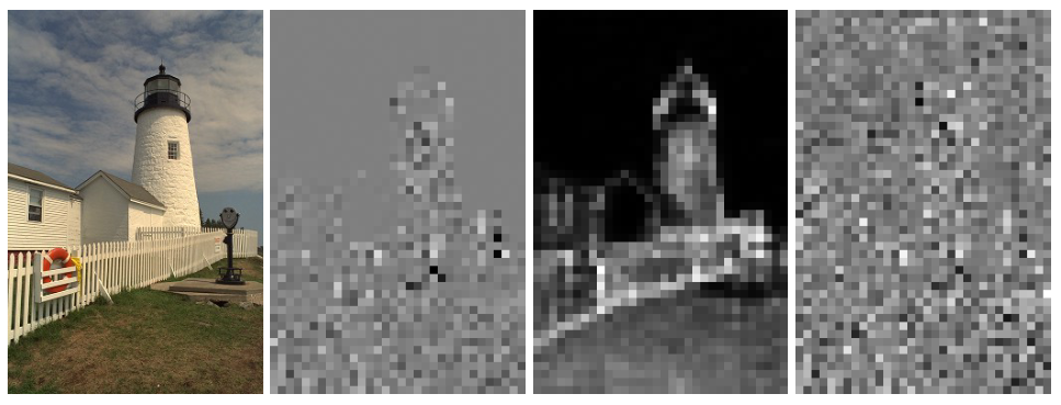
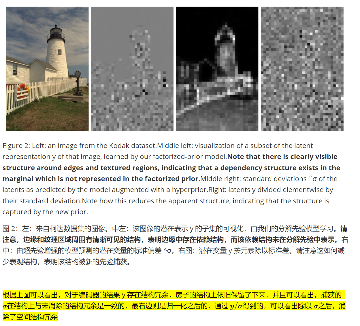
Figure 2: Left: an image from the Kodak dataset.Middle left: visualization of a subset of the latent representation y of that image, learned by our factorized-prior model.Note that there is clearly visible structure around edges and textured regions, indicating that a dependency structure exists in the marginal which is not represented in the factorized prior.Middle right: standard deviations ˆσ of the latents as predicted by the model augmented with a hyperprior.Right: latents y divided elementwise by their standard deviation.Note how this reduces the apparent structure, indicating that the structure is captured by the new prior.

图 2：左：来自柯达数据集的图像。中左：该图像的潜在表示 y 的子集的可视化，由我们的分解先验模型学习。请注意，边缘和纹理区域周围有清晰可见的结构，表明边缘中存在依赖结构，而该依赖结构未在分解先验中表示。右中：由超先验增强的模型预测的潜在变量的标准偏差 ^σ。右图：潜在变量 y 按元素除以标准差。请注意这如何减少表观结构，表明该结构被新的先验捕获。

根据上图可以看出，对于编码器的结果 y 存在结构冗余，房子的结构上依旧保留了下来，并且可以看出，捕获的 $\sigma$在结构上与未消除的结构冗余是一致的，最右边则是归一化之后的，通过 $y/\sigma$得到的，可以看出除以 $\sigma$之后，消除了空间结构冗余

In the transform coding approach to image compression (Goyal, 2001), the encoder transforms the image vector x using a parametric analysis transform ga(x; φg ) into a latent representation y, which is then quantized to form ˆy. Because ˆy is discrete-valued, it can be losslessly compressed using entropy coding techniques such as arithmetic coding (Rissanen and Langdon, 1981) and transmitted as a sequence of bits.On the other side, the decoder recovers ˆy from the compressed signal, and subjects it to aparametric synthesis transform gs(ˆy; θg ) to recover the reconstructed image ˆx.In the context of this paper, we think of the transforms ga and gs as generic parameterized functions, such as artificial neural networks (ANNs), rather than linear transforms asin traditional compression methods.The parameters θg and φg then encapsulate the weights of the neurons, etc. (refer to section 4 for details)

在图像压缩的变换编码方法中（Goyal，2001），编码器使用参数分析变换 ga(x; φg ) 将图像向量 x 变换为潜在表示 y，然后将其量化以形成 ˆy。因为 ˆy 是离散的-值，它可以使用算术编码（Rissanen 和 Langdon，1981）等熵编码技术进行无损压缩，并作为比特序列进行传输。 另一方面，解码器从压缩信号中恢复 ˆy，并将其置于参数综合变换 gs(ˆy; θg ) 来恢复重建图像 ˆx。在本文中，我们将变换 ga 和 gs 视为通用参数化函数，例如人工神经网络 (ANN)，而不是线性变换，如传统压缩方法中的参数θg和φg则封装了神经元的权重等（详细参考第4节）

The quantization introduces error, which is tolerated in the context of lossy compression, giving rise to a rate–distortion optimization problem.Rate is the expected code length (bit rate) of the compressed representation: assuming the entropy coding technique is operating efficiently, this can again be written as a cross entropy

量化引入了误差，该误差在有损压缩的情况下是可以容忍的，从而引起速率失真优化问题。速率是压缩表示的预期代码长度（比特率）：假设熵编码技术有效运行，这可以再次写为交叉熵

(2)

where Q represents the quantization function, and pˆy is the entropy model, as described in the in- troduction.In this context, the marginal distribution of the latent representation arises from the (unknown) image distribution px and the properties of the analysis transform.Distortion is the expected difference between the reconstruction ˆx and the original image x, as measured by a norm or perceptual metric.The coarseness of the quantization, or alternatively, the warping of the representation implied by the analysis and synthesis transforms, affects both rate and distortion, leading to a trade-off, where a higher rate allows for a lower distortion, and vice versa.Various compression methods can be viewed as minimizing a weighted sum of these two quantities.Formally, we can parameterize the problem by λ, a weight on the distortion term.Different applications require different trade-offs, and hence different values of λ.

其中 Q 表示量化函数，p^y 是熵模型，如引言中所述。在这种情况下，潜在表示的边缘分布由（未知）图像分布 px 和分析变换的属性产生。失真是重建图像 x 和原始图像 x 之间的预期差异，通过规范或感知度量来测量。量化的粗糙度，或者分析和合成变换所暗示的表示的扭曲，会影响速率和失真，从而导致一种权衡，即较高的速率允许较低的失真，反之亦然。各种压缩方法可以被视为最小化这两个量的加权和。形式上，我们可以通过 λ（失真项的权重）来参数化问题。不同的应用需要不同的权衡，因此需要不同的 λ 值。

In order to be able to use gradient descent methods to optimize the performance of the model over the parameters of the transforms (θg and φg ), the problem needs to be relaxed, because due to the quantization, gradients with respect to φg are zero almost everywhere. Approximations that have been investigated include substituting the gradient of the quantizer (Theis et al., 2017), and substituting additive uniform noise for the quantizer itself during training (Ballé et al., 2016b).Here, we follow the latter method,which switches back to actual quantization when applying the model as a compression method.We denote the quantities derived from this approximation with a tilde, as opposed to a hat;for instance, ̃y represents the “noisy” representation, and ˆy the quantized representation

为了能够使用梯度下降方法来优化模型在变换参数（θg 和 φg ）上的性能，需要放宽问题，因为由于量化，相对于 φg 的梯度几乎在任何地方都为零已经研究的近似包括替换量化器的梯度（Theis et al., 2017），以及在训练期间用加性均匀噪声替换量化器本身（Ballé et al., 2016b）。这里，我们遵循后一种方法，当将模型应用为压缩方法时，它会切换回实际量化。我们用波形符而不是帽子来表示从该近似值导出的量；例如， ̃y 表示“噪声”表示，而 ˆy 表示量化表示

The optimization problem can be formally represented as a variational autoencoder (Kingma and Welling, 2014);that is, a probabilistic generative model of the image combined with an approximate inference model (figure 1).The synthesis transform is linked to the generative model (“generating” a reconstructed image from the latent representation), and the analysis transform to the inference model (“inferring” the latent representation from the source image).In variational inference, the goal is to approximate the true posterior p ̃y|x(̃y | x), which is assumed intractable, with a para- metric variational density q( ̃y | x) by minimizing the expectation of their Kullback–Leibler (KL) divergence over the data distribution px

优化问题可以正式表示为变分自动编码器（Kingma 和 Welling，2014）；即图像的概率生成模型与近似推理模型相结合（图 1）。综合变换与生成模型相关联（从潜在表示“生成”重建图像），并将分析转换为推理模型（从源图像“推断”潜在表示）。在变分推理中，目标是逼近真实后验 p ̃y|x( ̃y | x)，假设这是棘手的，通过最小化数据分布 px 上的 Kullback-Leibler (KL) 散度的期望，得到参数变分密度 q( ̃y | x)

(3)

By matching the parametric density functions to the transform coding framework, we can appreciate that the minimization of the KL divergence is equivalent to optimizing the compression model for rate–distortion performance.We have indicated here that the first term will evaluate to zero, and the second and third term correspond to the weighted distortion and the bit rate, respectively.Let’s take a closer look at each of the terms.

通过将参数密度函数与变换编码框架相匹配，我们可以理解，KL 散度的最小化相当于优化压缩模型的率失真性能。我们在此指出，第一项的计算结果为零，第二项和第三项分别对应于加权失真和比特率。让我们仔细看看每个术语。

First, the mechanism of “inference” is computing the the analysis transform of the image and adding uniform noise (as a stand-in for quantization), thus:

首先，“推理”的机制是计算图像的分析变换并添加均匀噪声（作为量化的替代），因此：

(4)

where U denotes a uniform distribution centered on yi.Since the width of the uniform distribution is constant (equal to one), the first term in the KL divergence technically evaluates to zero, and can be dropped from the loss function.

其中 U 表示以 yi 为中心的均匀分布。由于均匀分布的宽度是恒定的（等于 1），因此 KL 散度中的第一项在技术上计算为零，并且可以从损失函数中删除。

For the sake of argument, assume for a moment that the likelihood is given by

为了便于论证，暂时假设可能性由下式给出

(5)

The log likelihood then works out to be the squared difference between x and ̃x, the output of the synthesis transform, weighted by λ.Minimizing the second term in the KL divergence is thus equivalent to minimizing the expected distortion of the reconstructed image.A squared error loss is equivalent to choosing a Gaussian distribution;other distortion metrics may have an equivalent distribution, but this is not guaranteed, as not all metrics necessarily correspond to a normalized density function

然后，对数似然计算为 x 和 ̃x 之间的平方差，即综合变换的输出，由 λ 加权。因此，最小化 KL 散度的第二项相当于最小化重建图像的预期失真。平方误差损失相当于选择高斯分布；其他失真度量可能具有等效分布，但这不能保证，因为并非所有度量都必须对应于归一化密度函数

The third term in the KL divergence is easily seen to be identical to the cross entropy between the marginal m( ̃y) = Ex∼px q( ̃y | x) and the prior p ̃y ( ̃y).It reflects the cost of encoding ̃y, as produced by the inference model, assuming p ̃y as the entropy model.Note that this term represents a differential cross entropy, as opposed to a Shannon (discrete) entropy as in eq.(2), due to the uniform noise approximation.Under the given assumptions, however, they are close approximations of each other (for an empirical evaluation of this approximation, see Ballé et al., 2017).Similarly to Ballé et al.(2017), we model the prior using a non-parametric, fully factorized density model (refer to appendix 6.1 for details)

KL 散度中的第三项很容易看出与边际 m( ̃y) = Ex∼px q( ̃y | x) 和先验 p ̃y ( ̃y) 之间的交叉熵相同。它反映了推理模型产生的编码 ̃y 的成本，假设 p ̃y 为熵模型。请注意，该术语表示微分交叉熵，而不是等式中的香农（离散）熵。 (2)、由于均匀噪声近似。然而，在给定的假设下，它们彼此非常近似（有关此近似值的实证评估，请参阅 Ballé 等人，2017）。与 Ballé 等人类似。 (2017)，我们使用非参数、完全分解的密度模型对先验进行建模（详细信息请参阅附录 6.1）

(6)

where the vectors ψ(i) encapsulate the parameters of each univariate distribution pyi|ψ(i) (we denote all these parameters collectively as ψ).Note that we convolve each non-parametric density with a standard uniform density.This is to enable a better match of the prior to the marginal – for more details, see appendix 6.2.As a shorthand, we refer to this case as the factorized-prior model

其中向量 ψ(i) 封装了每个单变量分布 pyi|ψ(i) 的参数（我们将所有这些参数统称为 ψ）。请注意，我们将每个非参数密度与标准均匀密度进行卷积。这是为了更好地匹配先验值和边际值——更多详细信息，请参见附录 6.2。作为简写，我们将这种情况称为分解先验模型

The center panel in figure 2 visualizes a subset of the quantized responses (ˆy) of a compression model trained in this way.Visually, it is clear that the choice of a factorized distribution is a stark simplification: non-zero responses are highly clustered in areas of high contrast;i.e., around edges, or within textured regions.This implies a probabilistic coupling between the responses, which is not represented in models with a fully factorized prior.We would expect a better model fit and, conse- quently, a better compression performance, if the model captured these dependencies.Introducing a hyperprior is an elegant way of achieving this.

图 2 中的中心面板可视化了以这种方式训练的压缩模型的量化响应 (ˆy) 的子集。从视觉上看，很明显，选择因式分解分布是一种明显的简化：非零响应高度聚集在高对比度区域；即，边缘周围或纹理区域内。这意味着响应之间存在概率耦合，而这种耦合在具有完全因式分解先验的模型中并未得到体现。如果模型捕获了这些依赖关系，我们预计会有更好的模型拟合，从而获得更好的压缩性能。引入超先验是实现这一目标的一种优雅方式

3 INTRODUCTION OF A SCALE HYPERPRIOR

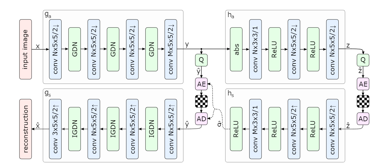
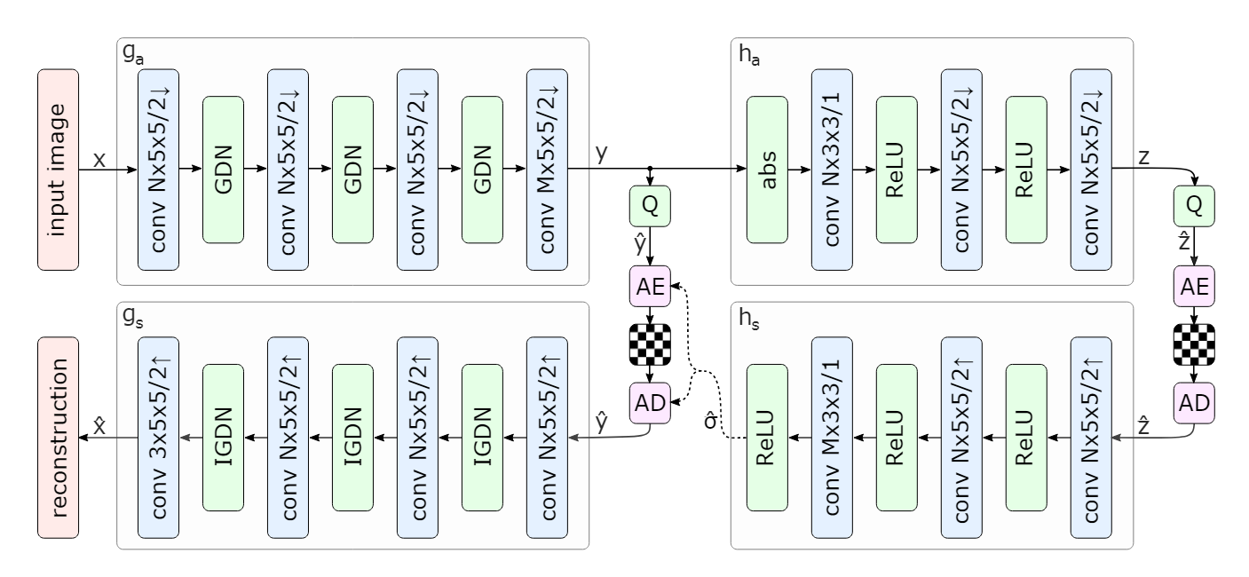
Figure 4: Network architecture of the hyperprior model.The left side shows an image autoen- coder architecture, the right side corresponds to the autoencoder implementing the hyperprior.The factorized-prior model uses the identical architecture for the analysis and synthesis transforms ga and gs.Q represents quantization, and AE, AD represent arithmetic encoder and arithmetic decoder, respectively.Convolution parameters are denoted as: number of filters × kernel support height × kernel support width / down- or upsampling stride, where ↑ indicates upsampling and ↓ downsam- pling.N and M were chosen dependent on λ, with N = 128 and M = 192 for the 5 lower values, and N = 192 and M = 320 for the 3 higher values

图 4：超先验模型的网络架构。左侧显示图像自动编码器架构，右侧对应于实现超先验的自动编码器。因式分解先验模型使用相同的架构来分析和综合变换 ga 和 gs。 Q表示量化，AE、AD分别表示算术编码器和算术解码器。卷积参数表示为：滤波器数量×内核支持高度×内核支持宽度/下采样或上采样步长，其中↑表示上采样，↓表示下采样。 N 和 M 的选择取决于 λ，对于 5 个较低值，N = 128 和 M = 192，对于 3 个较高值，N = 192 和 M = 320

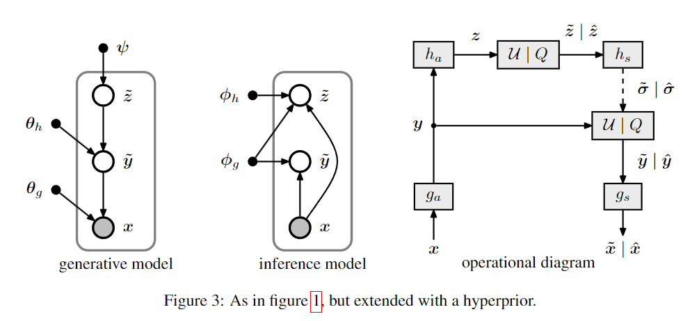
The right-hand panel in figure 3 illustrates how the model is used as a compression method.The encoder subjects the input image x to ga, yielding the responses y with spatially varying stan- dard deviations.The responses are fed into ha, summarizing thedistribution of standard deviations in z.z is then quantized, compressed, and transmitted as side information.The encoder then uses the quantized vector ˆz to estimate ˆσ, the spatial distribution of standard deviations, and uses it to compress and transmit the quantized image representation ˆy.The decoder first recovers ˆz from the compressed signal.It then uses hs to obtain ˆσ, which provides it with the correct probability estimates to successfully recover ˆy as well.It then feeds ˆy into gs to obtain the reconstructed image

图 3 的右侧面板说明了如何将模型用作压缩方法。编码器将输入图像 x 置于 ga 中，产生具有空间变化标准差的响应 y。响应被馈送到 ha，总结然后，z.z 中标准差的分布被量化、压缩并作为辅助信息传输。然后，编码器使用量化向量 ˆz 来估计 ˆσ（标准差的空间分布），并使用它来压缩和传输量化图像表示 ˆy。解码器首先从压缩信号中恢复 ˆz。然后使用 hs 获得 ˆσ，这为解码器提供了正确的概率估计以成功恢复 ˆy。然后将 ˆy 馈送到 gs 中以获得重建图像

个人总结

动机

基于香农定理，使用估计所得熵模型对隐层表示建模理论上的编码下界为：
KaTeX parse error: Got function '\hat' with no arguments as subscript at position 33: …m m}[-log_{2}p_\̲h̲a̲t̲ ̲y(\hat y)]
其中为m隐层表示（latent representation）实际分布,KaTeX parse error: Got function '\hat' with no arguments as subscript at position 3: p_\̲h̲a̲t̲ ̲y为熵模型估计分布，熵模型是一个发送人与接收人共享的先验概率模型，用来估计真实隐层表示分布。上面的式子说明当熵模型估计与实际分布完全相同的时候会有编码长度最小。这告诉我们，一方面，当熵模型使用全分解（fully factorized）概率分布的时候，如果实际分布中存在统计依赖，熵模型估计分布天然不能拟合实际分布；另一方面，因为y=enocde(x)是一个确定性的过程，如果想要在使用全分解概率分布的情况下效果提升，则需要encoder对输入的自然图像尽量多的去除统计依赖

如何理解"当熵模型使用全分解（fully factorized）概率分布的时候，如果实际分布中存在统计依赖，熵模型估计分布天然不能拟合实际分布"这句话

指的熵模型是 end-to-end image compression optimize那篇论文的熵模型

当我们使用熵模型（例如，变分自编码器或生成对抗网络）来估计概率分布时，如果我们假设该概率分布是全分解的，即可以表示为多个独立因子的乘积形式，但实际分布中存在统计依赖，那么熵模型将无法准确地拟合实际分布。

这是因为全分解概率分布假设了所有变量之间是独立的，而实际分布中可能存在变量之间的相关性或依赖关系。因此，当使用全分解概率分布时，熵模型无法捕捉到这些依赖关系，从而无法准确地表示实际分布。

什么是熵模型

熵模型（Entropy Model）是一种用于建模数据的概率分布的模型。它是基于信息论中的熵（entropy）概念而得名。

熵是衡量一个随机变量的不确定性的度量。在信息论中，熵越高表示随机变量的不确定性越大，越低表示不确定性越小。熵模型利用熵的概念来描述数据的概率分布，从而对数据进行建模和分析。

熵模型可以采用不同的形式和算法来建模数据的概率分布。常见的熵模型包括：

1. 参数化概率分布模型：例如高斯分布、伯努利分布等。这些模型通过参数化的方式定义概率分布，并通过最大似然估计等方法来学习参数。
2. 非参数化概率分布模型：例如核密度估计、混合模型等。这些模型不对概率分布进行具体参数化，而是通过对数据进行拟合来估计概率密度函数。
3. 生成模型：例如变分自编码器（Variational Autoencoder, VAE）、生成对抗网络（Generative Adversarial Networks, GAN）等。这些模型通过学习数据的潜在表示和生成过程来建模概率分布，并可以用于生成新的样本。

熵模型在机器学习和深度学习中被广泛应用于数据建模、生成、压缩等任务。它们提供了一种有效的方法来描述和学习数据的概率分布，从而可以进行各种有用的数据分析和处理。

这篇文章，关键在于引入辅助信息，捕捉隐层表示的隐藏信息以辅助熵模型的参数生成，从而改善熵模型估计与隐层实际分布不匹配问题。**将辅助信息导入比特流，这使得decoder也可以共享熵模型。**解压时decoder先解压边信息，构建熵模型，之后基于正确的熵模型解压隐层信息。

流程

Q表示量化，AE、AD分别表示算术编码器和算术解码器

输入图片经过主编码器 $g_a$ 获得了输出 y，即通过编码器得到的潜在特征表示，经过量化器 Q后得到输出$\hat{y}$
，超先验网络对 $\hat{y}$ 进行尺度（$\sigma$）捕获，对潜在表示每一个点进行均值为0，方差为 $ \sigma$ 的高斯建模，不同于以往的方法，以往的方式通过对整体潜在特征进行建模，即一个熵模型在推理阶段应用在所有的特征值熵，而超先验架构为每个特征点都进行了熵模型建模，通过对特征值的熵模型获取特征点的出现情况以用于码率估计和熵编码。

由于算术/范围编码器在编解码阶段都需要解码点的出现概率或者CDF（累计概率分布）表。故而需要将这部分信息传输到解码端，以用于正确的熵解码。故而超先验网络对这部分信息先压缩成 z,通过对 z 进行量化熵编码传输至超先验解码端，超先验解码端解码学习潜在表示 y 的建模参数。通过超先验网络获取得到潜在表示 y 的建模分布后，对其建模并且对量化后的 $\hat{y}$ 进行熵编码得到压缩后的码流文件，而通过熵解码得到 $ \hat{y}$ ，传统的编解码框架中往往设定反量化模块，而在解码网络中，包含了反量化的功能。故而在反量化模块在论文中并未部署，再将熵解码结果$\hat{y} $ 输入到主解码端，得到最终的重建图片 $ \hat{x} $。

  y = analysis_transform(x)  ##编码器
  z = hyper_analysis_transform(abs(y)) ##超先验编码获得z
  z_tilde, z_likelihoods = entropy_bottleneck(z, training=True)  ##对z进行量化，以及码率估计
  sigma = hyper_synthesis_transform(z_tilde) ##解码z，得到对应的sigma 参数，即方差
  scale_table = np.exp(np.linspace(
      np.log(SCALES_MIN), np.log(SCALES_MAX), SCALES_LEVELS)) ##构建分组边界
  conditional_bottleneck = tfc.GaussianConditional(sigma, scale_table) ##实例化高斯分布的熵率模型
  y_tilde, y_likelihoods = conditional_bottleneck(y, training=True) ##量化y，以及估计y的码率
  x_tilde = synthesis_transform(y_tilde) ##根据量化后的值，重构图像

思路

全文思路建立在编码器提取潜在特征的特征存在一定的结构冗余（如上图所示），这部分结构冗余即一些像素点存在相关性，本文的思路即如何消除这部分的相关性