ZFNet论文阅读

ZFNet论文阅读

Visualizing and Understanding Convolutional Networks
参考资料：https://blog.csdn.net/qq_39297053/article/details/130667098
简介：

ZFNet其实跟AlexNet很像很像， 首先是ZFNet改变了AlexNet的第一层，将卷积核的尺寸从11×11变为7×7，并将步长从4变为2。这一微小的修改就显著地改进了整个卷积神经网络的性能，使ZFNet在2013年ImageNet图像分类竞赛中获得了冠军。

单词

不重要的

corresponding 相应的

mask out 掩盖

重要的

ablation study 消融实验 即对比实验

unsupervised learning 无监督学习

unPooling 反池化

Filtering 过滤 ，视频上说是卷积的别称，不过好像有点区别

(62条消息) 卷积核（kernel）和过滤器（filter）的区别_卷积核和过滤器是一样的吗_Medlen的博客-CSDN博客

convnet 即CNN

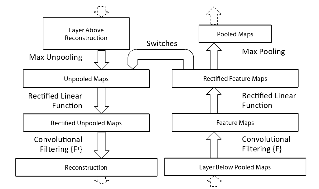
反池化（unPooling）

the max pooling operation is non-invertible, however we can obtain an approximate inverse by recording the locations of the maxima within each pooling region in a set of switch variables

最大池操作是不可逆的，但是我们可以通过在一组开关变量中记录每个池区域内最大值的位置来获得近似逆

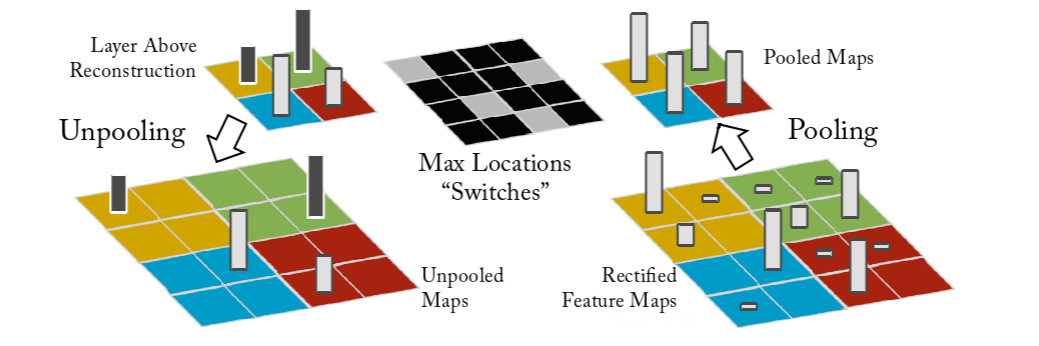
如上图所示，右下角是池化操作，获得pooled Maps，然后把最大值位置信息记录在Max Location "Switches"中，在图中用灰色来表示。这样就能返回Unpooled Maps了

为什么说是近似？因为这样只能把池化后的结果返回，其他的都没了(通过看源码，发现其他直接赋值0)

• The convnet uses relu non-linearities, which rectify the feature maps thus ensuring the feature maps are always positive.To obtain valid feature reconstructions at each layer (which also should be positive), we pass the reconstructed signal through a relu non-linearity

• convnet 使用 relu 非线性，校正特征图从而确保特征图始终为正。为了在每一层获得有效的特征重建（也应该是正的），我们通过 relu 非线性传递重建信号。

• The convnet uses learned filters to convolve the feature maps from the previous layer.To approximately invert this, the deconvnet uses transposed versions of the same filters (as other autoencoder models, such as RBMs), but applied to the rectified maps, not the output of the layer beneath.In practice this means flipping each filter vertically and horizontally.

• convnet 使用学习过滤器对来自上一层的特征图进行卷积。为了近似地反转它，deconvnet 使用相同过滤器的转置版本（作为其他自动编码器模型，例如 RBM），但应用于校正映射，而不是下面层的输出。实际上，这意味着垂直和水平翻转每个过滤器。

如下图所示，大致流程是先反池化，然后用relu函数确保为正，最后做反卷积

卷积结果可视化

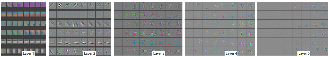
一项重要的实验是将卷积核的计算结果映射回原始的像素空间（映射的方法为反卷积，反池化）并进行可视化。例如，以Layer 1为例，左上角的九宫格代表第一层卷积计算得到的前九张特征图映射回原图像素空间后的可视化（称为F9）。第一层卷积使用96个卷积核，这意味着会得到96张特征图，这里的前九张特征图是指96个卷积核中值最大的9个卷积核对应生成的特征图（这里称这9个卷积核为K9，即，第一层卷积最关注的前九种特征）。可以发现，这九种特征都是颜色和纹理特征，即蕴含语义信息少的结构性特征。
为了证明这个观点，将数据集中的原始图像裁剪成小图，将所有的小图送进网络中，得到第一层卷积计算后的特征图。统计能使K9中每个卷积核输入计算结果最大的前9张输入小图，即9×9=81张，如图右下角所示。结果表明刚刚可视化的F9和这81张小图表征的特征是相似的，且一一对应的。由此证明卷积网络在第一层提取到的是一些颜色，纹理特征。

The projections from each layer show the hierarchical nature of the features in the network.Layer 2 responds to corners and other edge/color conjunctions.Layer 3 has more complex invariances, capturing similar textures (e.g. mesh patterns (Row 1, Col 1); text (R2,C4)).Layer 4 shows significant variation, and is more class-specific: dog faces (R1,C1);bird’s legs (R4,C2).Layer 5 shows entire objects with significant pose variation, e.g.keyboards (R1,C11) and dogs (R4).

每层的投影显示了网络中特征的层次结构。
第 2 层响应角和其他边缘/颜色连接。
第 3 层具有更复杂的不变性，捕获相似的纹理（例如网格图案（第 1 行，第 1 列）；文本（R2，C4））。
第 4 层显示出显着的变化，并且更具体：狗脸（R1，C1）；鸟的腿（R4，C2）。
第 5 层显示具有显着姿势变化的整个对象，例如键盘（R1，C11）和狗（R4）。

最后，越靠近输出端，能激活卷积核的输入图像相关性越少（尤其是空间相关性），例如Layer5中，最右上角的示例：feature map中表征的是一种绿色成片的特征，可是能激活这些特征的原图相关性却很低（因为原图是人，马，海边，公园等，语义上并不相干）；其实这种绿色成片的特征是‘草地’，而这些语义不相干的图片里都有‘草地’。‘草地’是网络深层卷积核提取的是高级语义信息，不再是低级的像素信息，空间信息等等。

• For example, in layer 5, row 1, col 2, the patches appear to have little in common, but the visualizations reveal that this particular feature map focuses on the grass in the background, not the foreground objects

• 例如，在第 5 层，第 1 行，第 2 列，这些补丁似乎没有什么共同之处，但可视化显示这个特定的特征图关注背景中的草地，而不是前景对象。

总结一下：CNN输出的特征图有明显的层级区分。

越靠近输入端，提取的特征所蕴含的语义信息比较少，例如颜色特征，边缘特征，角点特征等等；

越靠近输出端，提取的特征所蕴含的语义信息越丰富，例如Layer4中的狗脸，鸟腿等，都属于目标级别的特征

网络对不同特征的学习速度

如下图所示，横轴表示训练轮数，纵轴表示不同层的feature maps映射回像素空间后的可视化结果：

总结：low-level的特征(颜色，纹理等)在网络训练的训练前期就可以学习到， 即更容易收敛；high-level的语义特征在网络训练的后期才会逐渐学到。 由此展示了不同特征的进化过程。这也是一个合理的过程，毕竟高级的语义特征，要在低级特征的基础上学习提取才能得到。

就比如第一层，训练一开始就能得到一些纹理的特征，而且在训练后半段得到的可视化结果是一样的（即更容易收敛）。而在第五层，训练一开始feature map是空的。

图片平移、缩放、旋转对CNN的影响

Analysis of vertical translation, scale, and rotation invariance within the model (rows a-c respectively).Col 1: 5 example images undergoing the transformations.Col 2 & 3: Euclidean distance between feature vectors from the original and transformed images in layers 1 and 7 respectively.Col 4: the probability of the true label for each image, as the image is transformed.

模型内的垂直平移、比例和旋转不变性分析（分别为 a-c 行）。
Col 1：5 个示例图像正在经历转换。
Col 2和Col 3：分别来自第 1 层和第 7 层中的原始图像和变换图像的特征向量之间的欧氏距离。
Col 4：随着图像的转换，每个图像的真实标签的概率。

欧式距离：

两点间的直线距离，根号下a方加b方。欧氏距离其实就是L2范数

• Feature Invariance: Fig. 5 shows 5 sample images being translated, rotated and scaled by varying degrees while looking at the changes in the feature vectors from the top and bottom layers of the model, relative to the untransformed feature.Small transformations have a dramatic effect in the first layer of the model, but a lesser impact at the top feature layer, being quasi- linear for translation & scaling.The network output is stable to translations and scalings.In general, the output is not invariant to rotation, except for object with rotational symmetry (e.g. entertainment center).

• 特征不变性：图 5 显示了 5 个样本图像被不同程度地平移、旋转和缩放，同时查看模型顶层和底层的特征向量相对于未变换特征的变化。小的变换对模型的第一层有显著影响，但对顶层特征层的影响较小，对于平移和缩放是准线性的。网络输出对于平移和缩放是稳定的。一般来说，输出不是旋转不变的，除了具有旋转对称性的物体（例如娱乐中心）。

个人理解：

1. 小的变换对模型的第一层有显著影响，但对顶层特征层的影响较小

   首先从图中可以看出第一层随着左右平移，得到的距离都会陡增或陡减。而第七层卷积的增减曲线变换平缓。这一定程度上说明了网络的深层提取的是高级语义特征，而不是低级的颜色，纹理，空间特征。高级语义信息不会随着平移操作而轻易改变。就比如狗的图片，你平移后肯定还是狗，但是如果你是一个纹理图，平移前后的变化就大了。

总结：卷积拥有良好的平移不变性和缩放不变性。 不具有良好的旋转不变性。

遮挡对卷积模型的影响

Deep models differ from many existing recognition ap- proaches in that there is no explicit mechanism for establishing correspondence between specific object parts in different images (e.g. faces have a particular spatial configuration of the eyes and nose).However, an intriguing possibility is that deep models might be implicitly computing them.

深度模型不同于许多现有的识别方法，因为没有明确的机制来建立不同图像中特定对象部分之间的对应关系（例如，面部具有特定的眼睛和鼻子空间配置）。然而，一个有趣的可能性是深度模型可能正在隐式计算它们。

b表示计算遮挡后的图像经过第五个卷积层后得到的feature map 值的总和。红色代表更大的值。 由此可以看出来卷积计算后的特征图也是保留了原始数据中不同类别对象在图像中的空间信息。

解释：就拿第一个图来说，图像中蓝色的区域位于动物面部。而这个图片的特征肯定是动物面部。所以feature map的总和就小了。

c左上角的小图是经过第五个卷积后值最大的特征图的deconv可视化结果。由此实例2（可视化结果为英文字母或汉字，但是原图标签的“车轮”）可以看出卷积后值最大的特征图不一定是对分类最有作用的。c中的其他小图是统计数据集中其他图像可以使该卷积核输出最大特征图的deconv可视化结果。

d表示灰色滑块所遮挡的位置对图像正确分类的影响，红色代表分类成功的可能性大。例如博美犬的图像，当灰色滑块遮挡到博美犬的面部时，模型对博美犬的识别准确率大幅度下降。

e表示模型对遮挡后的图像的分类结果是什么。还拿博美犬的例子，灰色遮挡在图片中非狗脸的位置时，都不影响模型将其正确分类为博美犬（大部分都是蓝色标签，除了遮挡滑动到狗脸位置时）。

这个遮挡实验证明，模型确实可以理解图片，找到语义信息最丰富，对识别最关键的特征；而不是仅仅依靠一些颜色，纹理特征去做识别。

此外，模型还做了进一步的遮挡实验来证明卷积可以提取到高级的语义特征，如下图所示：

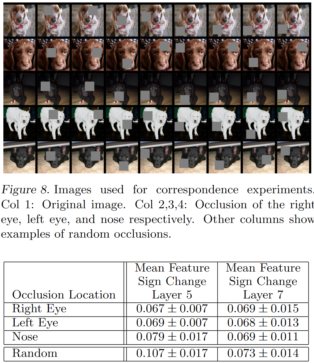
通过遮挡图像的不同部位来证明CNN在处理图像的时候是关注局部的高级语义特征，而不是根据图像的全部信息来处理。

例如第二列遮挡左眼，表中的结果是求这五种不同狗 Dpair 的Hamming distance之和，即：Dpair是原图和遮挡图，Hamming distance是分别送进CNN中得到的feature map的差值之和。

数值越小表面遮挡左眼这个操作对不同种类的狗起到的作用是差不多的。

表中随机遮挡的结果（最后一列）明显大于有规律的遮挡，因此反应了CNN确实隐式对不同类别的同种特征做了学习总结。

值得注意的是，Layer7的随机遮挡结果明显小于Layer5，这说明深层的网络提取的是语义信息（例如狗的类属），而不是low-level的空间特征。因此对随机遮挡可以不敏感。

汉明距离

在信息论中，两个等长字符串之间的汉明距离（英语：Hamming distance）是两个字符串对应位置的不同字符的个数。换句话说，它就是将一个字符串变换成另外一个字符串所需要替换的字符个数。

如果将这两个数用二进制表示的话，有a=1011101、b=1001001，可以看出，二者的从右往左数的第3位、第5位不同（从1开始数），因此，a和b的汉明距离是2。

代码

ZFnet

import torch.nn as nn
import torch
from torchsummary import summary

# 与AlexNet有两处不同： 1. 第一次的卷积核变小，步幅减小。 2. 第3，4，5层的卷积核数量增加了。
class ZFNet(nn.Module):
    def __init__(self, num_classes=1000, init_weights=False):
        super(ZFNet, self).__init__()
        self.features = nn.Sequential(
            nn.Conv2d(3, 96, kernel_size=7, stride=2, padding=2),  # input[3, 224, 224]  output[96, 111, 111]
            nn.ReLU(inplace=True),
            nn.MaxPool2d(kernel_size=3, stride=2),                  # output[96, 55, 55]

            nn.Conv2d(96, 256, kernel_size=5, padding=2),           # output[256, 55, 55]
            nn.ReLU(inplace=True),
            nn.MaxPool2d(kernel_size=3, stride=2),                  # output[256, 27, 27]

            nn.Conv2d(256, 512, kernel_size=3, padding=1),          # output[512, 27, 27]
            nn.ReLU(inplace=True),

            nn.Conv2d(512, 1024, kernel_size=3, padding=1),          # output[1024, 27, 27]
            nn.ReLU(inplace=True),

            nn.Conv2d(1024, 512, kernel_size=3, padding=1),          # output[512, 27, 27]
            nn.ReLU(inplace=True),
            nn.MaxPool2d(kernel_size=3, stride=2),                  # output[512, 13, 13]
        )
        self.classifier = nn.Sequential(
            nn.Dropout(p=0.5),
            nn.Linear(512 * 13 * 13, 4096),
            nn.ReLU(inplace=True),

            nn.Dropout(p=0.5),
            nn.Linear(4096, 4096),
            nn.ReLU(inplace=True),
            
            nn.Linear(4096, num_classes),
        )
        if init_weights:
            self._initialize_weights()

    def forward(self, x):
        x = self.features(x)
        x = torch.flatten(x, start_dim=1)
        x = self.classifier(x)
        return x

    def _initialize_weights(self):
        for m in self.modules():
            if isinstance(m, nn.Conv2d):
                nn.init.kaiming_normal_(m.weight, mode='fan_out', nonlinearity='relu')
                if m.bias is not None:
                    nn.init.constant_(m.bias, 0)
            elif isinstance(m, nn.Linear):
                nn.init.normal_(m.weight, 0, 0.01)
                nn.init.constant_(m.bias, 0)

def zfnet(num_classes): 
    model = ZFNet(num_classes=num_classes)
    return model

# net = ZFNet(num_classes=1000)
# summary(net.to('cuda'), (3,224,224))
#########################################################################################################################################
# Total params: 386,548,840
# Trainable params: 386,548,840
# Non-trainable params: 0
# ----------------------------------------------------------------
# Input size (MB): 0.57
# Forward/backward pass size (MB): 57.77
# Params size (MB): 1474.57
# Estimated Total Size (MB): 1532.91
# ----------------------------------------------------------------
# conv_parameters:  11,247,744 相比于AelxNet的cnn层参数  3,747,200   增加 3 倍
# fnn_parameters:  375,301,096 相比于AelxNet的fnn层参数 58,631,144   增加 6.4 倍
# 卷积参数占全模型参数的 2% ；全连接层占 98%