


🍨 本文为🔗365天深度学习训练营中的学习记录博客
🍖 原作者:K同学啊 | 接辅导、项目定制
🚀 文章来源:K同学的学习圈子
此次学习的重点:
(1)学习YOLO-C3模块,并比较不同数量下的C3模块对训练结果的test_acc有何影响;
- 模型每增加一个C3模块,
forward()函数内部也同步增加一个C3模块;这是因为init里是定义,forward是调用
1.环境配置
import torch
import torch.nn as nn
import torchvision.transforms as transforms
import torchvision
from torchvision import transforms, datasets
import os,PIL,pathlib,warnings

warnings.filterwarnings("ignore")             #忽略警告信息

device = torch.device("cuda" if torch.cuda.is_available() else "cpu")
device
import os,PIL,random,pathlib
data_dir = './8-data/'
data_dir = pathlib.Path(data_dir)
data_paths = list(data_dir.glob('*'))
classeNames = [str(path).split("\\")[1] for path in data_paths]
classeNames
# 关于transforms.Compose的更多介绍可以参考:https://blog.csdn.net/qq_38251616/article/details/124878863
train_transforms = transforms.Compose([
transforms.Resize([224, 224]), # 将输入图片resize成统一尺寸
# transforms.RandomHorizontalFlip(), # 随机水平翻转
transforms.ToTensor(), # 将PIL Image或numpy.ndarray转换为tensor,并归一化到[0,1]之间
transforms.Normalize( # 标准化处理-->转换为标准正太分布(高斯分布),使模型更容易收敛
mean=[0.485, 0.456, 0.406],
std=[0.229, 0.224, 0.225]) # 其中 mean=[0.485,0.456,0.406]与std=[0.229,0.224,0.225] 从数据集中随机抽样计算得到的。
])
test_transform = transforms.Compose([
transforms.Resize([224, 224]), # 将输入图片resize成统一尺寸
transforms.ToTensor(), # 将PIL Image或numpy.ndarray转换为tensor,并归一化到[0,1]之间
transforms.Normalize( # 标准化处理-->转换为标准正太分布(高斯分布),使模型更容易收敛
mean=[0.485, 0.456, 0.406],
std=[0.229, 0.224, 0.225]) # 其中 mean=[0.485,0.456,0.406]与std=[0.229,0.224,0.225] 从数据集中随机抽样计算得到的。
])
total_data = datasets.ImageFolder("./8-data/",transform=train_transforms)
total_data2.划分数据集
train_size = int(0.8 * len(total_data))
test_size  = len(total_data) - train_size
train_dataset, test_dataset = torch.utils.data.random_split(total_data, [train_size, test_size])
train_dataset, test_dataset
batch_size = 4

train_dl = torch.utils.data.DataLoader(train_dataset,
                                           batch_size=batch_size,
                                           shuffle=True,
                                           num_workers=1)
test_dl = torch.utils.data.DataLoader(test_dataset,
                                          batch_size=batch_size,
                                          shuffle=True,
                                          num_workers=1)
3.搭建包含C3模块的模型
import torch.nn.functional as F
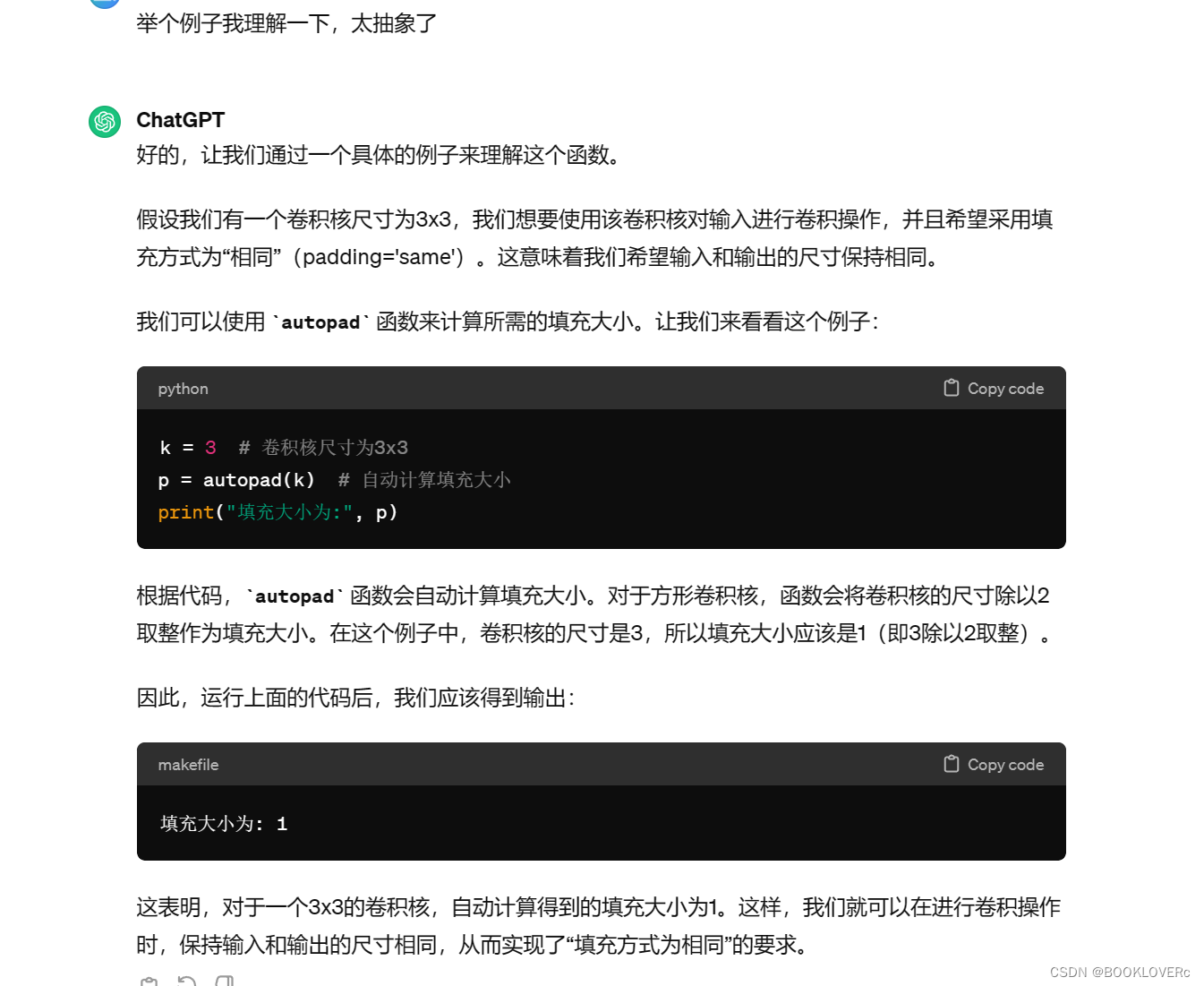
def autopad(k, p=None): # kernel, padding
# Pad to 'same'
if p is None:
p = k // 2 if isinstance(k, int) else [x // 2 for x in k] # auto-pad
return p在判断语句中,首先检查卷积核的尺寸 k 是否为整数。如果是整数,表示 k 是一个方形卷积核,其宽度和高度相同。在这种情况下,使用卷积核的尺寸 k 的一半作为填充大小。
-
如果
k是整数,执行k // 2将卷积核尺寸除以2取整,得到的值作为填充大小。 -
如果卷积核的尺寸
k不是整数,表示k是一个由两个整数组成的列表,分别表示卷积核的宽度和高度。在这种情况下,分别计算每个维度的填充大小,将它们组成一个列表。 -
返回计算得到的填充大小
p。
这个函数实现了一个常见的机制,即“自动填充(auto-padding)”,它使得在进行卷积操作时,可以通过简单地传入卷积核的尺寸,自动计算所需的填充大小以保持输入与输出的尺寸相同,这通常用于卷积神经网络中的“填充方式为相同(padding='same')”的情况。
让GPT举了个例子方便我具体理解这个函数
class Conv(nn.Module):
    # Standard convolution
    def __init__(self, c1, c2, k=1, s=1, p=None, g=1, act=True):  # ch_in, ch_out, kernel, stride, padding, groups
        super().__init__()
        self.conv = nn.Conv2d(c1, c2, k, s, autopad(k, p), groups=g, bias=False)
        self.bn = nn.BatchNorm2d(c2)
        self.act = nn.SiLU() if act is True else (act if isinstance(act, nn.Module) else nn.Identity())
这段代码的作用是创建一个卷积层,并在卷积后应用批标准化和激活函数,构成了一个标准的卷积层组件。
class Bottleneck(nn.Module):
    # Standard bottleneck
    def __init__(self, c1, c2, shortcut=True, g=1, e=0.5):  # ch_in, ch_out, shortcut, groups, expansion
        super().__init__()
        c_ = int(c2 * e)  # hidden channels
        self.cv1 = Conv(c1, c_, 1, 1)
        self.cv2 = Conv(c_, c2, 3, 1, g=g)
        self.add = shortcut and c1 == c2

    def forward(self, x):
        return x + self.cv2(self.cv1(x)) if self.add else self.cv2(self.cv1(x))
这段代码定义了一个名为 Bottleneck 的类,该类表示了一个标准的瓶颈(Bottleneck)块
class C3(nn.Module):
    # CSP Bottleneck with 3 convolutions
    def __init__(self, c1, c2, n=1, shortcut=True, g=1, e=0.5):  # ch_in, ch_out, number, shortcut, groups, expansion
        super().__init__()
        c_ = int(c2 * e)  # hidden channels
        self.cv1 = Conv(c1, c_, 1, 1)
        self.cv2 = Conv(c1, c_, 1, 1)
        self.cv3 = Conv(2 * c_, c2, 1)  # act=FReLU(c2)
        self.m = nn.Sequential(*(Bottleneck(c_, c_, shortcut, g, e=1.0) for _ in range(n)))

    def forward(self, x):
        return self.cv3(torch.cat((self.m(self.cv1(x)), self.cv2(x)), dim=1))
本周重点(C3模块):
这段代码定义了一个名为 C3 的类,表示了一个具有3次卷积操作的CSP瓶颈(CSP Bottleneck)。这个类通过使用CSP(Cross-Stage Partial Connections)结构来提高模型的表达能力。
创建三个卷积层 self.cv1、self.cv2 和 self.cv3,分别用于CSP瓶颈中的三次卷积操作。这三个卷积层分别是:
self.cv1:一个1x1的卷积层,用于减少通道数。self.cv2:一个1x1的卷积层,用于减少通道数。self.cv3:一个1x1的卷积层,用于在减少通道数后再次增加通道数。
创建一个由多个 Bottleneck 块组成的序列,这些 Bottleneck 块共享相同的输入和输出通道数,即 c_。
在前向传播方法中,首先通过第一个卷积层 self.cv1 对输入 x 进行卷积操作,然后通过 Bottleneck 块序列 self.m 对第一个卷积层的输出进行多次卷积操作。接着,将第一个卷积层和 Bottleneck 块序列的输出通过 torch.cat() 函数进行拼接,然后再通过第二个卷积层 self.cv2 进行卷积操作。最后,通过第三个卷积层 self.cv3 进行卷积操作,并返回其结果。
class model_K(nn.Module):
    def __init__(self):
        super(model_K, self).__init__()

        # 卷积模块
        self.Conv = Conv(3, 32, 3, 2)

        # C3模块1
        self.C3_1 = C3(32, 64, 3, 2)

        # 全连接网络层,用于分类
        self.classifier = nn.Sequential(
            nn.Linear(in_features=802816, out_features=100),
            nn.ReLU(),
            nn.Linear(in_features=100, out_features=4)
        )
总的模型串联
总的模型信息是
----------------------------------------------------------------
        Layer (type)               Output Shape         Param #
================================================================
            Conv2d-1         [-1, 32, 112, 112]             864
       BatchNorm2d-2         [-1, 32, 112, 112]              64
              SiLU-3         [-1, 32, 112, 112]               0
              Conv-4         [-1, 32, 112, 112]               0
            Conv2d-5         [-1, 32, 112, 112]           1,024
       BatchNorm2d-6         [-1, 32, 112, 112]              64
              SiLU-7         [-1, 32, 112, 112]               0
              Conv-8         [-1, 32, 112, 112]               0
            Conv2d-9         [-1, 32, 112, 112]           1,024
      BatchNorm2d-10         [-1, 32, 112, 112]              64
             SiLU-11         [-1, 32, 112, 112]               0
             Conv-12         [-1, 32, 112, 112]               0
           Conv2d-13         [-1, 32, 112, 112]           9,216
      BatchNorm2d-14         [-1, 32, 112, 112]              64
             SiLU-15         [-1, 32, 112, 112]               0
             Conv-16         [-1, 32, 112, 112]               0
       Bottleneck-17         [-1, 32, 112, 112]               0
           Conv2d-18         [-1, 32, 112, 112]           1,024
      BatchNorm2d-19         [-1, 32, 112, 112]              64
             SiLU-20         [-1, 32, 112, 112]               0
             Conv-21         [-1, 32, 112, 112]               0
           Conv2d-22         [-1, 32, 112, 112]           9,216
      BatchNorm2d-23         [-1, 32, 112, 112]              64
             SiLU-24         [-1, 32, 112, 112]               0
             Conv-25         [-1, 32, 112, 112]               0
       Bottleneck-26         [-1, 32, 112, 112]               0
           Conv2d-27         [-1, 32, 112, 112]           1,024
      BatchNorm2d-28         [-1, 32, 112, 112]              64
             SiLU-29         [-1, 32, 112, 112]               0
             Conv-30         [-1, 32, 112, 112]               0
           Conv2d-31         [-1, 32, 112, 112]           9,216
      BatchNorm2d-32         [-1, 32, 112, 112]              64
             SiLU-33         [-1, 32, 112, 112]               0
             Conv-34         [-1, 32, 112, 112]               0
       Bottleneck-35         [-1, 32, 112, 112]               0
           Conv2d-36         [-1, 32, 112, 112]           1,024
      BatchNorm2d-37         [-1, 32, 112, 112]              64
             SiLU-38         [-1, 32, 112, 112]               0
             Conv-39         [-1, 32, 112, 112]               0
           Conv2d-40         [-1, 64, 112, 112]           4,096
      BatchNorm2d-41         [-1, 64, 112, 112]             128
             SiLU-42         [-1, 64, 112, 112]               0
             Conv-43         [-1, 64, 112, 112]               0
               C3-44         [-1, 64, 112, 112]               0
           Linear-45                  [-1, 100]      80,281,700
             ReLU-46                  [-1, 100]               0
           Linear-47                    [-1, 4]             404
================================================================
Total params: 80,320,536
Trainable params: 80,320,536
Non-trainable params: 0
----------------------------------------------------------------
Input size (MB): 0.57
Forward/backward pass size (MB): 150.06
Params size (MB): 306.40
Estimated Total Size (MB): 457.04
----------------------------------------------------------------
4.训练函数和测试函数
# 训练循环
def train(dataloader, model, loss_fn, optimizer):
    size = len(dataloader.dataset)  # 训练集的大小
    num_batches = len(dataloader)   # 批次数目, (size/batch_size,向上取整)

    train_loss, train_acc = 0, 0  # 初始化训练损失和正确率

    for X, y in dataloader:  # 获取图片及其标签
        X, y = X.to(device), y.to(device)

        # 计算预测误差
        pred = model(X)          # 网络输出
        loss = loss_fn(pred, y)  # 计算网络输出和真实值之间的差距,targets为真实值,计算二者差值即为损失

        # 反向传播
        optimizer.zero_grad()  # grad属性归零
        loss.backward()        # 反向传播
        optimizer.step()       # 每一步自动更新

        # 记录acc与loss
        train_acc  += (pred.argmax(1) == y).type(torch.float).sum().item()
        train_loss += loss.item()

    train_acc  /= size
    train_loss /= num_batches

    return train_acc, train_loss

def test (dataloader, model, loss_fn):
    size        = len(dataloader.dataset)  # 测试集的大小
    num_batches = len(dataloader)          # 批次数目, (size/batch_size,向上取整)
    test_loss, test_acc = 0, 0

    # 当不进行训练时,停止梯度更新,节省计算内存消耗
    with torch.no_grad():
        for imgs, target in dataloader:
            imgs, target = imgs.to(device), target.to(device)

            # 计算loss
            target_pred = model(imgs)
            loss        = loss_fn(target_pred, target)

            test_loss += loss.item()
            test_acc  += (target_pred.argmax(1) == target).type(torch.float).sum().item()

    test_acc  /= size
    test_loss /= num_batches

    return test_acc, test_loss
5.正式训练
import copy

optimizer  = torch.optim.Adam(model.parameters(), lr= 1e-4)
loss_fn    = nn.CrossEntropyLoss() # 创建损失函数

epochs     = 20

train_loss = []
train_acc  = []
test_loss  = []
test_acc   = []

best_acc = 0    # 设置一个最佳准确率,作为最佳模型的判别指标

for epoch in range(epochs):

    model.train()
    epoch_train_acc, epoch_train_loss = train(train_dl, model, loss_fn, optimizer)

    model.eval()
    epoch_test_acc, epoch_test_loss = test(test_dl, model, loss_fn)

    # 保存最佳模型到 best_model
    if epoch_test_acc > best_acc:
        best_acc   = epoch_test_acc
        best_model = copy.deepcopy(model)

    train_acc.append(epoch_train_acc)
    train_loss.append(epoch_train_loss)
    test_acc.append(epoch_test_acc)
    test_loss.append(epoch_test_loss)

    # 获取当前的学习率
    lr = optimizer.state_dict()['param_groups'][0]['lr']

    template = ('Epoch:{:2d}, Train_acc:{:.1f}%, Train_loss:{:.3f}, Test_acc:{:.1f}%, Test_loss:{:.3f}, Lr:{:.2E}')
    print(template.format(epoch+1, epoch_train_acc*100, epoch_train_loss,
                          epoch_test_acc*100, epoch_test_loss, lr))

# 保存最佳模型到文件中
PATH = './best_model.pth'  # 保存的参数文件名
torch.save(model.state_dict(), PATH)

print('Done')
Epoch: 1, Train_acc:70.4%, Train_loss:1.143, Test_acc:84.4%, Test_loss:0.967, Lr:1.00E-04
Epoch: 2, Train_acc:86.3%, Train_loss:0.389, Test_acc:84.9%, Test_loss:1.085, Lr:1.00E-04
Epoch: 3, Train_acc:89.8%, Train_loss:0.332, Test_acc:84.9%, Test_loss:1.764, Lr:1.00E-04
Epoch: 4, Train_acc:92.8%, Train_loss:0.232, Test_acc:85.3%, Test_loss:1.321, Lr:1.00E-04
Epoch: 5, Train_acc:95.8%, Train_loss:0.141, Test_acc:84.9%, Test_loss:1.471, Lr:1.00E-04
Epoch: 6, Train_acc:97.4%, Train_loss:0.079, Test_acc:86.2%, Test_loss:1.066, Lr:1.00E-04
Epoch: 7, Train_acc:97.4%, Train_loss:0.065, Test_acc:83.6%, Test_loss:1.534, Lr:1.00E-04
Epoch: 8, Train_acc:97.8%, Train_loss:0.079, Test_acc:84.0%, Test_loss:1.226, Lr:1.00E-04
Epoch: 9, Train_acc:98.9%, Train_loss:0.034, Test_acc:88.0%, Test_loss:0.973, Lr:1.00E-04
Epoch:10, Train_acc:96.7%, Train_loss:0.139, Test_acc:86.7%, Test_loss:1.064, Lr:1.00E-04
Epoch:11, Train_acc:97.3%, Train_loss:0.088, Test_acc:86.2%, Test_loss:1.316, Lr:1.00E-04
Epoch:12, Train_acc:98.9%, Train_loss:0.038, Test_acc:88.9%, Test_loss:0.681, Lr:1.00E-04
Epoch:13, Train_acc:99.6%, Train_loss:0.015, Test_acc:86.2%, Test_loss:0.928, Lr:1.00E-04
Epoch:14, Train_acc:99.2%, Train_loss:0.040, Test_acc:82.7%, Test_loss:1.446, Lr:1.00E-04
Epoch:15, Train_acc:98.9%, Train_loss:0.024, Test_acc:83.6%, Test_loss:0.941, Lr:1.00E-04
Epoch:16, Train_acc:99.6%, Train_loss:0.014, Test_acc:88.4%, Test_loss:0.953, Lr:1.00E-04
Epoch:17, Train_acc:99.8%, Train_loss:0.007, Test_acc:88.0%, Test_loss:1.068, Lr:1.00E-04
Epoch:18, Train_acc:99.2%, Train_loss:0.025, Test_acc:86.7%, Test_loss:1.290, Lr:1.00E-04
Epoch:19, Train_acc:98.9%, Train_loss:0.033, Test_acc:85.3%, Test_loss:1.073, Lr:1.00E-04
Epoch:20, Train_acc:99.6%, Train_loss:0.016, Test_acc:88.4%, Test_loss:1.267, Lr:1.00E-04
Done测试集准确率达到了88.4%
6.结果可视化
import matplotlib.pyplot as plt
#隐藏警告
import warnings
warnings.filterwarnings("ignore")               #忽略警告信息
plt.rcParams['font.sans-serif']    = ['SimHei'] # 用来正常显示中文标签
plt.rcParams['axes.unicode_minus'] = False      # 用来正常显示负号
plt.rcParams['figure.dpi']         = 100        #分辨率

epochs_range = range(epochs)

plt.figure(figsize=(12, 3))
plt.subplot(1, 2, 1)

plt.plot(epochs_range, train_acc, label='Training Accuracy')
plt.plot(epochs_range, test_acc, label='Test Accuracy')
plt.legend(loc='lower right')
plt.title('Training and Validation Accuracy')

plt.subplot(1, 2, 2)
plt.plot(epochs_range, train_loss, label='Training Loss')
plt.plot(epochs_range, test_loss, label='Test Loss')
plt.legend(loc='upper right')
plt.title('Training and Validation Loss')
plt.show()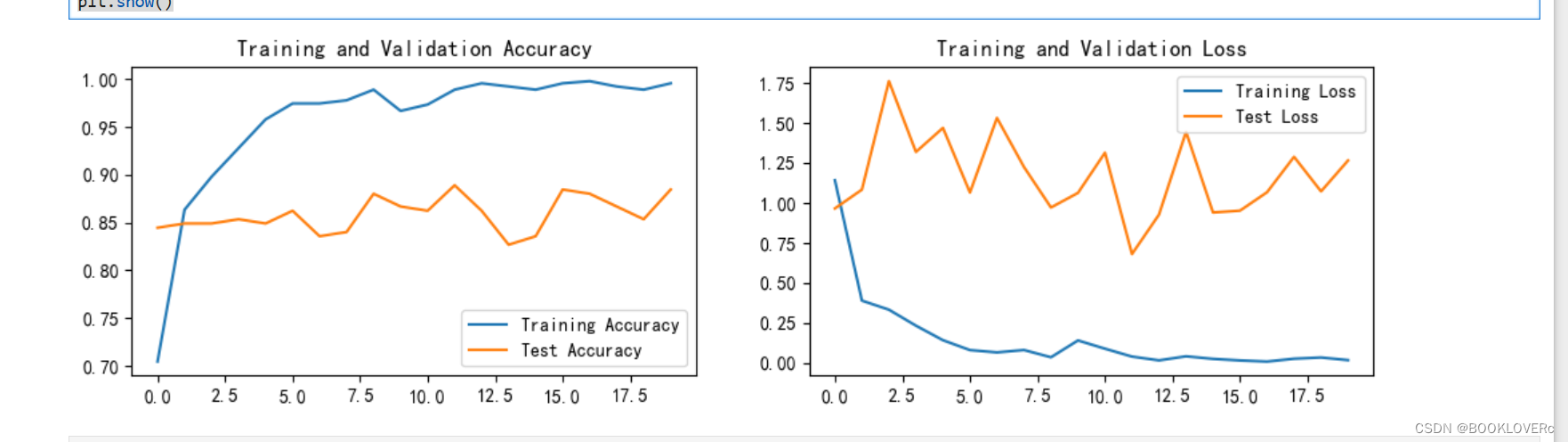


 406
406


 被折叠的 条评论
为什么被折叠?
被折叠的 条评论
为什么被折叠?
 到【灌水乐园】发言


