第R2周：LSTM-火灾温度预测

本文为🔗365天深度学习训练营中的学习记录博客
🍖 原作者：K同学啊 | 接辅导、项目定制
🚀 文章来源：K同学的学习圈子

 

1.对LSTM的理解

LSTM，全称为长短期记忆网络(Long Short Term Memory networks)，是一种特殊的RNN，能够学习到长期依赖关系。LSTM由Hochreiter & Schmidhuber (1997)提出，许多研究者进行了一系列的工作对其改进并使之发扬光大。LSTM在许多问题上效果非常好，现在被广泛使用。
LSTM是为了避免长依赖问题而精心设计的。 记住较长的历史信息实际上是他们的默认行为，而不是他们努力学习的东西。
遗忘门: 控制上一时间步的记忆细胞;
输入门:控制当前时间步的输入;
输出门:控制从记忆细胞到隐藏状态;
记忆细胞：⼀种特殊的隐藏状态的信息的流动,表示的是长期记忆;
h 是隐藏状态，表示的是短期记忆;

所有的循环神经网络都有着重复的神经网络模块形成链的形式。在普通的RNN中，重复模块结构非常简单，其结构如下：

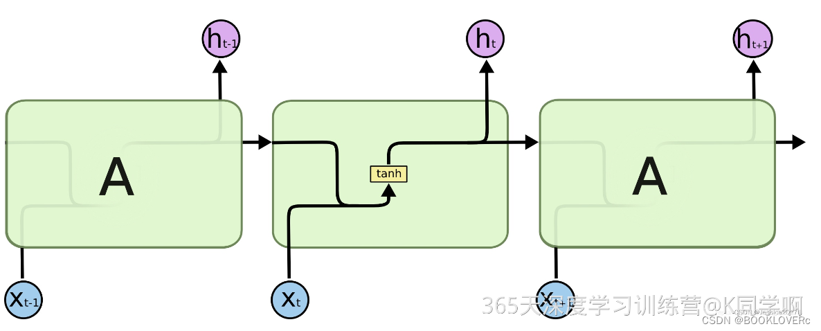
LSTM避免了长期依赖的问题。可以记住长期信息！LSTM内部有较为复杂的结构。能通过门控状态来选择调整传输的信息，记住需要长时间记忆的信息，忘记不重要的信息，其结构如下：

2.数据准备

import numpy as np
import pandas as pd
import torch
from torch import nn
import torch.nn.functional as F
from torch.utils.data import TensorDataset, DataLoader
data = pd.read_csv("./dataRnn2/woodpine2.csv")
print(data.head(5))
print(data.columns)

   Time  Tem1  CO 1  Soot 1
0  0.000  25.0   0.0     0.0
1  0.228  25.0   0.0     0.0
2  0.456  25.0   0.0     0.0
3  0.685  25.0   0.0     0.0
4  0.913  25.0   0.0     0.0
Index(['Time', 'Tem1', 'CO 1', 'Soot 1'], dtype='object')

输出前五列

import matplotlib.pyplot as plt
import seaborn as sns
 
plt.rcParams['savefig.dpi'] = 500 #图片像素
plt.rcParams['figure.dpi']  = 500 #分辨率
 
fig, ax =plt.subplots(1,3,constrained_layout=True, figsize=(14, 3))
 
sns.lineplot(data=data["Tem1"], ax=ax[0])
sns.lineplot(data=data["CO 1"], ax=ax[1])
sns.lineplot(data=data["Soot 1"], ax=ax[2])
plt.show()

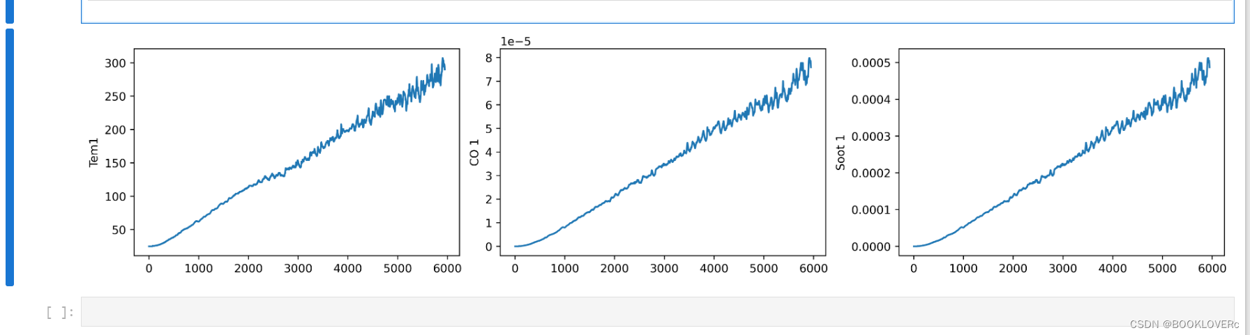
数据集原始数据随时间变化情况

dataFrame = data.iloc[:,1:]
dataFrame

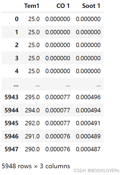
dataFrame = data.iloc[:,1:].copy()
## 归一化
from sklearn.preprocessing import MinMaxScaler
col=[ 'CO 1', 'Soot 1', 'Tem1']
#将数据归一化，范围是0到1
sc       = MinMaxScaler(feature_range=(0, 1))
for i in col:
    dataFrame[i] = sc.fit_transform(dataFrame[i].values.reshape(-1, 1))
print(dataFrame.shape)

###设置X、y
width_X = 8
width_y = 2
##取前8个时间段的Tem1、CO 1、Soot 1为X，第9个时间段的Tem1为y。
X = []
y = []

in_start = 0

for _, _ in data.iterrows():
    in_end  = in_start + width_X
    out_end = in_end   + width_y
    
    if out_end < len(dataFrame):
        X_ = np.array(dataFrame.iloc[in_start:in_end , ])
        #X_ = X_.reshape((len(X_)*3))
        y_ = np.array(dataFrame.iloc[in_end  :out_end, 0])

        X.append(X_)
        y.append(y_)
    
    in_start += 1

X = np.array(X)
y = np.array(y).reshape(-1,1,2)

X.shape, y.shape

1. 首先，通过 data.iloc[:,1:].copy() 选择了数据中除第一列外的所有列，将其存储在 dataFrame 变量中。这里使用 .copy() 方法是为了确保生成一个新的数据框，而不是对原始数据进行修改。

2. 接着，通过 MinMaxScaler 对选定的列进行了归一化处理，这些列是 'CO 1', 'Soot 1', 'Tem1'。归一化的范围被限制在 0 到 1 之间。

3. 然后，设置了输入和输出的宽度，分别为 width_X = 8 和 width_y = 2。

4. 通过循环遍历数据中的每一行，并以每行数据的前8个时间段的 'CO 1', 'Soot 1', 'Tem1' 作为输入 X，第9个时间段的 'Tem1' 作为输出 y。这里通过移动窗口的方式来获取输入和输出数据。

5. 在循环过程中，根据输入和输出的宽度以及当前的起始位置，从 dataFrame 中选择对应的数据，并将其加入到 X 和 y 中。其中，X 是一个三维数组，y 是一个二维数组。

6. 最后，将 X 和 y 转换为 NumPy 数组，并输出它们的形状。

print(np.any(np.isnan(X)))
print(np.any(np.isnan(y)))

检查数据集中是否有空值

X_train = torch.tensor(np.array(X[:5000]), dtype=torch.float32)
y_train = torch.tensor(np.array(y[:5000]), dtype=torch.float32)

X_test  = torch.tensor(np.array(X[5000:]), dtype=torch.float32)
y_test  = torch.tensor(np.array(y[5000:]), dtype=torch.float32)
X_train.shape

取5000之前的数据为训练集，5000之后的为验证集

train_dl = DataLoader(TensorDataset(X_train, y_train),batch_size=64, shuffle=False)
test_dl = DataLoader(TensorDataset(X_test, y_test),batch_size=64, shuffle=False)

3.模型构建

*LSTM **

LSTM接收数据形式为input_size=(batce_size,seq_length,input_size)此处input_size=out_channels，将维度交换有：
input_size=(batch_size,seq_length,out_channels)

LSTM输出结果维度形式为：
output=(batch_size, seq_len, num_directions * hidden_size)

全连接层的输入维度形式为：
fc=(hidden_size,output_size)

LSTM隐层状态h0, c0通常初始化为0，大部分情况下模型也能工作的很好。
LSTM的隐藏层初始状态h0, c0可以看做是模型的一部分参数，并在迭代中更新

class model_lstm(nn.Module):
    def __init__(self):
        super(model_lstm, self).__init__()
        self.lstm0 = nn.LSTM(input_size=3 ,hidden_size=320, num_layers=1, batch_first=True)
        self.lstm1 = nn.LSTM(input_size=320 ,hidden_size=320, num_layers=1, batch_first=True)
        self.fc0 = nn.Sequential(nn.Linear(320, 300),nn.Dropout(0.3))
        self.fc1 = nn.Sequential(nn.Linear(300, 2))
 
    def forward(self, x):
 
        #h_0 = torch.randn(1, x.size(0), 64)  #num_layers * num_directions(单向/双向), bs，hidden_size
        #c_0 = torch.randn(1, x.size(0), 64)  #num_layers * num_directions(单向/双向), bs，hidden_size
        #如果不传入h0和c0，pytorch会将其初始化为0
 
        out, hidden1 = self.lstm0(x) 
        out, _ = self.lstm1(out, hidden1) 
        out = self.fc0(out) 
        out = self.fc1(out) 
        return out[:, -1:, :]   #取2个预测值,否则经过lstm会得到8*2个预测
'''
def init_weight(model):
    for m in model.modules():
        if isinstance(m, nn.Linear):
            torch.nn.init.uniform_(m.weight.data, a=0, b=1)
'''  
model = model_lstm()
#model.apply(init_weight)
model
 

4.模型训练

#设置GPU训练
device=torch.device("cuda" if torch.cuda.is_available() else "cpu")
 
# 训练循环
import copy
def train(train_dl, model, loss_fn, opt, lr_scheduler=None):
    size = len(train_dl.dataset)  
    num_batches = len(train_dl)   
    train_loss = 0  # 初始化训练损失和正确率
    
    for x, y in train_dl:  
        x, y = x.to(device), y.to(device)
        
        # 计算预测误差
        #pred = model(x)
        pred = model(x)          # 网络输出
        loss = loss_fn(pred, y)  # 计算网络输出和真实值之间的差距
        
        # 反向传播
        opt.zero_grad()  # grad属性归零
        loss.backward()        # 反向传播
        opt.step()       # 每一步自动更新
        
        # 记录loss
        train_loss += loss.item()
    if lr_scheduler is not None:
        lr_scheduler.step()
        print("learning rate = ", opt.param_groups[0]['lr'])
    train_loss /= num_batches
    return train_loss
 
def test (dataloader, model, loss_fn):
    size        = len(dataloader.dataset)  # 测试集的大小
    num_batches = len(dataloader)          # 批次数目
    test_loss = 0
    
    # 当不进行训练时，停止梯度更新，节省计算内存消耗
    with torch.no_grad():
        for x, y in dataloader:
            
            x, y = x.to(device), y.to(device)
            
            # 计算loss
            y_pred = model(x)
            loss        = loss_fn(y_pred, y)
            test_loss += loss.item()
        
    test_loss /= num_batches
    return test_loss

#训练模型
model = model_lstm()
model = model.to(device)
loss_fn    = nn.MSELoss() # 创建损失函数
learn_rate = 1e-1   # 学习率
opt        = torch.optim.SGD(model.parameters(),lr=learn_rate,weight_decay=1e-4)
epochs     = 150
train_loss = []
test_loss  = []
lr_scheduler = torch.optim.lr_scheduler.CosineAnnealingLR(opt,epochs, last_epoch=-1) 
best_val =[0, 1e5]
for epoch in range(epochs):
    model.train()
    epoch_train_loss = train(train_dl, model, loss_fn, opt, lr_scheduler)
 
    model.eval()
    epoch_test_loss = test(test_dl, model, loss_fn)
    if best_val[1] >  epoch_test_loss:
        best_val =[epoch, epoch_test_loss]
        best_model_wst = copy.deepcopy(model.state_dict())
 
    train_loss.append(epoch_train_loss)
    test_loss.append(epoch_test_loss)
    
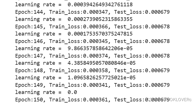
    template = ('Epoch:{:2d}, Train_loss:{:.6f}, Test_loss:{:.6f}')
    print(template.format(epoch+1, epoch_train_loss,  epoch_test_loss))
print("*"*20, 'Done', "*"*20)
print("best_train= ", best_train)

5.模型评估

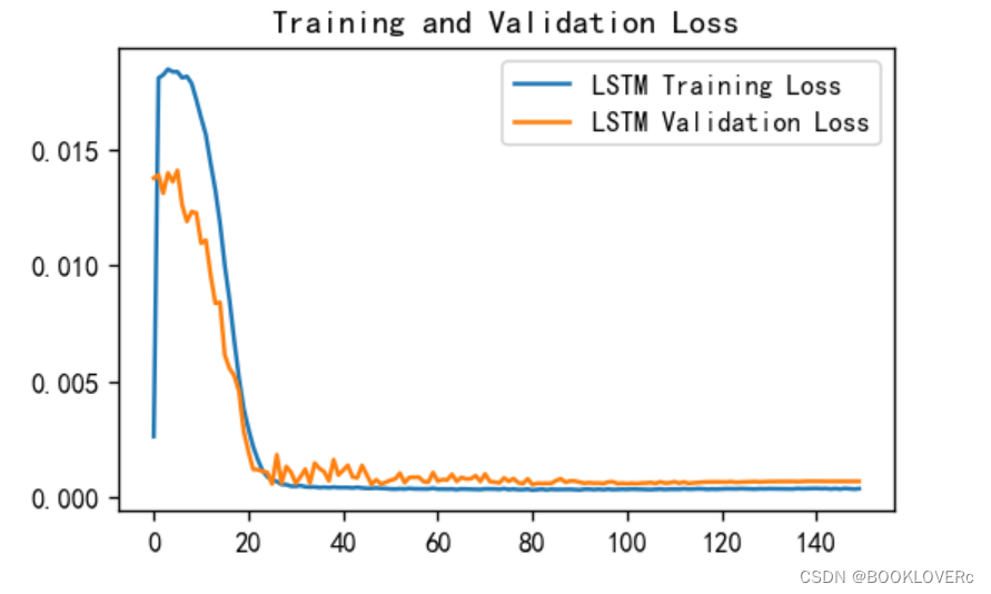
#LOSS图
# 支持中文
import matplotlib.pyplot as plt
plt.rcParams['font.sans-serif'] = ['SimHei']  # 用来正常显示中文标签
plt.rcParams['axes.unicode_minus'] = False  # 用来正常显示负号
 
plt.figure(figsize=(5, 3),dpi=120)
 
plt.plot(train_loss    , label='LSTM Training Loss')
plt.plot(test_loss, label='LSTM Validation Loss')
 
plt.title('Training and Validation Loss')
plt.legend()
plt.show()

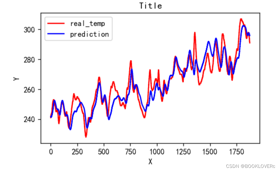
预测

model.load_state_dict(best_model_wst)
model.to("cpu")
predicted_y_lstm = sc.inverse_transform(model(X_test).detach().numpy().reshape(-1,1))                    # 测试集输入模型进行预测
y_test_1 = sc.inverse_transform(y_test.reshape(-1,1))
y_test_one = [i[0] for i in y_test_1]
predicted_y_lstm_one = [i[0] for i in predicted_y_lstm]
 
plt.figure(figsize=(5, 3),dpi=120)
# 画出真实数据和预测数据的对比曲线
plt.plot(y_test_one[:2000], color='red', label='real_temp')
plt.plot(predicted_y_lstm_one[:2000], color='blue', label='prediction')
 
plt.title('Title')
plt.xlabel('X')
plt.ylabel('Y')
plt.legend()
plt.show()

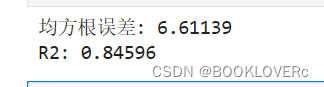
from sklearn import metrics
"""
RMSE ：均方根误差  ----->  对均方误差开方
R2   ：决定系数，可以简单理解为反映模型拟合优度的重要的统计量
"""
RMSE_lstm  = metrics.mean_squared_error(predicted_y_lstm_one, y_test_1)**0.5
R2_lstm    = metrics.r2_score(predicted_y_lstm_one, y_test_1)
 
print('均方根误差: %.5f' % RMSE_lstm)
print('R2: %.5f' % R2_lstm)

test_1 = torch.tensor(dataFrame.iloc[:8 , ].values,dtype = torch.float32).reshape(1,-1,3)
pred_ = model(test_1)
pred_ = np.round(sc.inverse_transform(pred_.detach().numpy().reshape(1,-1)).reshape(-1),2)
real_tem = data.Tem1.iloc[:2].values
print(f"第9~10时刻的温度预测：",  pred_)
print("第9~10时刻的真实温度：",  real_tem)