2021-07-23

深度学习应用

1 深度学习完成垃圾分类任务

1.1背景介绍

该任务是基于MindSpore框架完成的，MindSpore是华为的一个AI开源框架，平行于PyTorch和TesnsorFlow，但是基本语法都差不多，因此用起来上手相对方便。深度学习中从头开始训练一个模型非常耗时耗力，因此我们经常采用的一种方法是：在一些经常用的数据集如OpenImage、ImageNet、VOC、COCO上采用已经预训练好的模型，做一些微调，来提升模型的效果，称为Fine Tune。

本实验以MobileNetV2+垃圾分类数据集为例，主要介绍如何使用MindSpore在CPU/GPU平台上进行Fine-Tune。

1.2 数据集介绍

一共有26种垃圾，分为干垃圾，可回收垃圾，湿垃圾，有害垃圾，我们需要做的事情是：给出一张图片，预测出它在26种垃圾中是哪一类，进而再根据下述对应关系将其分类。

{
    '干垃圾': ['贝壳', '打火机', '旧镜子', '扫把', '陶瓷碗', '牙刷', '一次性筷子', '脏污衣服'],
    '可回收物': ['报纸', '玻璃制品', '篮球', '塑料瓶', '硬纸板', '玻璃瓶', '金属制品', '帽子', '易拉罐', '纸张'],
    '湿垃圾': ['菜叶', '橙皮', '蛋壳', '香蕉皮'],
    '有害垃圾': ['电池', '药片胶囊', '荧光灯', '油漆桶']
}

['贝壳', '打火机', '旧镜子', '扫把', '陶瓷碗', '牙刷', '一次性筷子', '脏污衣服',
'报纸', '玻璃制品', '篮球', '塑料瓶', '硬纸板', '玻璃瓶', '金属制品', '帽子', '易拉罐', '纸张',
'菜叶', '橙皮', '蛋壳', '香蕉皮',
'电池', '药片胶囊', '荧光灯', '油漆桶']

['Seashell', 'Lighter', 'Old Mirror', 'Broom', 'Ceramic Bowl', 'Toothbrush', 'Disposable Chopsticks', 'Dirty Cloth',
'Newspaper', 'Glassware', 'Basketball', 'Plastic Bottle', 'Cardboard', 'Glass Bottle', 'Metalware', 'Hats', 'Cans', 'Paper',
'Vegetable Leaf', 'Orange Peel', 'Eggshell', 'Banana Peel',
'Battery', 'Tablet capsules', 'Fluorescent lamp', 'Paint bucket']

1.3 实验正式开始

预处理

首先我们需要导入需要用到的包

import math
import numpy as np
import os
import cv2
import random
import shutil
import time
from matplotlib import pyplot as plt
from easydict import EasyDict
from PIL import Image
# mindspore是和pytorch平行的另一套框架
import mindspore as ms
from mindspore import context
from mindspore import nn
from mindspore import Tensor
from mindspore.train.model import Model
from mindspore.train.serialization import load_checkpoint, save_checkpoint, export
from mindspore.train.callback import Callback, LossMonitor, ModelCheckpoint, CheckpointConfig

from src_mindspore.dataset import create_dataset # 数据处理脚本
from src_mindspore.mobilenetv2 import MobileNetV2Backbone, mobilenet_v2 # 模型定义脚本

os.environ['GLOG_v'] = '2' # Log Level = Error
has_gpu = (os.system('command -v nvidia-smi') == 0)
print('Excuting with', 'GPU' if has_gpu else 'CPU', '.')
context.set_context(mode=context.GRAPH_MODE, device_target='GPU' if has_gpu else 'CPU')

然后我们将26种垃圾依次编码，并且预先设定超参。深度学习很大一项工作是调参（又称炼丹），调的就是超参数。在这个网络中我们需要调整以下五个主要超参：

1. "epochs": 4, # 请尝试修改以提升精度，需要调整
2. "lr_max": 0.01, # 请尝试修改以提升精度，需要调整
3. "decay_type": 'constant', # 请尝试修改以提升精度，需要调整
4. "momentum": 0.8, # 请尝试修改以提升精度，需要调整
5. "weight_decay": 3.0, # 请尝试修改以提升精度，需要调整

# 垃圾分类数据集标签，以及用于标签映射的字典。
# 00_00代表可回收物，01_00代表干垃圾，02_00代表有害垃圾，03_00代表湿垃圾
index = {'00_00': 0, '00_01': 1, '00_02': 2, '00_03': 3, '00_04': 4, '00_05': 5, '00_06': 6, '00_07': 7,
         '00_08': 8, '00_09': 9, '01_00': 10, '01_01': 11, '01_02': 12, '01_03': 13, '01_04': 14, 
         '01_05': 15, '01_06': 16, '01_07': 17, '02_00': 18, '02_01': 19, '02_02': 20, '02_03': 21,
         '03_00': 22, '03_01': 23, '03_02': 24, '03_03': 25}
inverted = {0: 'Plastic Bottle', 1: 'Hats', 2: 'Newspaper', 3: 'Cans', 4: 'Glassware', 5: 'Glass Bottle', 6: 'Cardboard', 7: 'Basketball',
            8: 'Paper', 9: 'Metalware', 10: 'Disposable Chopsticks', 11: 'Lighter', 12: 'Broom', 13: 'Old Mirror', 14: 'Toothbrush',
            15: 'Dirty Cloth', 16: 'Seashell', 17: 'Ceramic Bowl', 18: 'Paint bucket', 19: 'Battery', 20: 'Fluorescent lamp', 21: 'Tablet capsules',
            22: 'Orange Peel', 23: 'Vegetable Leaf', 24: 'Eggshell', 25: 'Banana Peel'}

# 训练超参
config = EasyDict({
    "num_classes": 26, # 分类数，即输出层的维度，一共26种垃圾
    "reduction": 'mean', # mean, max, Head部分池化采用的方式，采用平均池化方式
    "image_height": 224, # 图像的高度
    "image_width": 224, # 图像的宽度
    "batch_size": 24, # 鉴于CPU容器性能，太大可能会导致训练卡住，batch_size=24
    "eval_batch_size": 10, # 这个是什么意思？
    "epochs": 4, # 请尝试修改以提升精度，需要调整
    "lr_max": 0.01, # 请尝试修改以提升精度，需要调整
    "decay_type": 'constant', # 请尝试修改以提升精度，需要调整
    "momentum": 0.8, # 请尝试修改以提升精度，需要调整
    "weight_decay": 3.0, # 请尝试修改以提升精度，需要调整
    "dataset_path": "./datasets/5fbdf571c06d3433df85ac65-momodel/garbage_26x100",# 垃圾数据集分类，训练集中每种垃圾提供100个例子，测试集每种垃圾提供5个样例
    "features_path": "./results/garbage_26x100_features", # 临时目录，保存冻结层Feature Map，可随时删除，标签集
    "class_index": index, # index是垃圾分类字典
    "save_ckpt_epochs": 1,
    "save_ckpt_path": './results/ckpt_mobilenetv2',
    "pretrained_ckpt": './src_mindspore/mobilenetv2-200_1067_cpu_gpu.ckpt',
    "export_path": './results/mobilenetv2.mindir'
    
})

训练策略

通常情况下，我们会采用静态学习率，如设置 , 但是由于随着模型的训练，参数会逐渐收敛，此时更新权重应该减小，所以可以采用动态学习率的方式，常用的有以下四种：

1. polynomial decay/square decay;
2. cosine decay;
3. exponential decay;
4. stage decay.

下面的代码给出了cosine decay和square decay的方式

def build_lr(total_steps, lr_init=0.0, lr_end=0.0, lr_max=0.1, warmup_steps=0, decay_type='cosine'):
    """
    Applies cosine decay to generate learning rate array.
    Args:
       total_steps(int): all steps in training.
       lr_init(float): init learning rate.
       lr_end(float): end learning rate
       lr_max(float): max learning rate.
       warmup_steps(int): all steps in warmup epochs.
    Returns:
       list, learning rate array.返回一个列表，告诉每步的学习率为多大
    """
    lr_init, lr_end, lr_max = float(lr_init), float(lr_end), float(lr_max)
    decay_steps = total_steps - warmup_steps
    lr_all_steps = []
    inc_per_step = (lr_max - lr_init) / warmup_steps if warmup_steps else 0
    for i in range(total_steps):
        if i < warmup_steps:
            lr = lr_init + inc_per_step * (i + 1)
        else:
            if decay_type == 'cosine':
                cosine_decay = 0.5 * (1 + math.cos(math.pi * (i - warmup_steps) / decay_steps))
                lr = (lr_max - lr_end) * cosine_decay + lr_end
            elif decay_type == 'square':
                frac = 1.0 - float(i - warmup_steps) / (total_steps - warmup_steps)
                lr = (lr_max - lr_end) * (frac * frac) + lr_end
            else:
                lr = lr_max
        lr_all_steps.append(lr)
    return lr_all_steps

我们可以从下图中直观的观察到三种学习率策略的不同

steps = 5*93
plt.plot(range(steps), build_lr(steps, lr_max=0.1, decay_type='constant'))
plt.plot(range(steps), build_lr(steps, lr_max=0.1, decay_type='square'))
plt.plot(range(steps), build_lr(steps, lr_max=0.1, decay_type='cosine'))
plt.show()

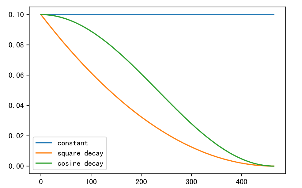
square decay 的学习率相比 cosine decay 下降地更快，但最后都几乎趋于0.

模型训练

在模型训练过程中，可以添加检查点（Checkpoint）用于保存模型的参数，以便进行推理及中断后再训练使用。使用场景如下：

• 训练后推理场景

  • 模型训练完毕后保存模型的参数，用于推理或预测操作。
  • 训练过程中，通过实时验证精度，把精度最高的模型参数保存下来，用于预测操作。
• 再训练场景

  • 进行长时间训练任务时，保存训练过程中的Checkpoint文件，防止任务异常退出后从初始状态开始训练。
  • Fine-tuning（微调）场景，即训练一个模型并保存参数，基于该模型，面向第二个类似任务进行模型训练。

这里加载 ImageNet 数据上预训练的 MobileNetv2进行Fine-tuning，并在训练过程中保存Checkpoint。训练有两种方式：

• 方式一：冻结网络的Backbone，只训练修改的FC层（Head）。其中，Backbone在全量数据集上做一遍推理，得到Feature Map，将Feature Map作为训练Head的数据集，可以极大节省训练时间。
• 方式二：先冻结网络的Backbone，只训练网络Head；再对Backbone+Head整网做微调。

这里的Backbone是什么意思呢？backbone愿意是 “脊梁骨（支柱）” 的意思，通常也就是指图像进行特征提取的部分，经过 backbone 部分会得到特征图，将特征图送入到全连接网络（称为Head部分，或修改层），我们只需训练Head部分的参数。

提取特征集

下面我们将冻结层在全量训练集上做一遍推理，然后保存 Feature Map，作为修改层的输入数据集。

def extract_features(net, dataset_path, config):
    if not os.path.exists(config.features_path):
        os.makedirs(config.features_path)
    dataset = create_dataset(config=config)
    step_size = dataset.get_dataset_size()
    if step_size == 0:
        raise ValueError("The step_size of dataset is zero. Check if the images count of train dataset is more \
            than batch_size in config.py")

    data_iter = dataset.create_dict_iterator()
    for i, data in enumerate(data_iter):
        features_path = os.path.join(config.features_path, f"feature_{i}.npy")
        label_path = os.path.join(config.features_path, f"label_{i}.npy")
        if not os.path.exists(features_path) or not os.path.exists(label_path):
            image = data["image"]
            label = data["label"]
            features = net(image)
            np.save(features_path, features.asnumpy())
            np.save(label_path, label.asnumpy())
        print(f"Complete the batch {i+1}/{step_size}")
    return

backbone = MobileNetV2Backbone() # 这里采用预先做好的Backbone
load_checkpoint(config.pretrained_ckpt, net=backbone)
extract_features(backbone, config.dataset_path, config)# 直接得到特征图，再对特征图做训练即可

训练Head层

首先定义一个全局池化的类（Class）

class GlobalPooling(nn.Cell):
    """
    Global avg pooling definition.全局平均池化
    Args:
        reduction: mean or max, which means AvgPooling or MaxpPooling.平均池化和最大值池化
    Returns:
        Tensor, output tensor.
    Examples:
        >>> GlobalAvgPooling()
    """
    def __init__(self, reduction='mean'):
        super(GlobalPooling, self).__init__()
        if reduction == 'max': # 最大值池化
            self.mean = ms.ops.ReduceMax(keep_dims=False)
        else: # 平均池化
            self.mean = ms.ops.ReduceMean(keep_dims=False)
    def construct(self, x):
        x = self.mean(x, (2, 3))
        return x

接下来我们定义 Head 层的结构：

class MobileNetV2Head(nn.Cell): 
    """
    MobileNetV2Head architecture. # 定义Head部分的结构
    Args:
        input_channel (int): Number of channels of input.
        hw (int): Height and width of input, 7 for MobileNetV2Backbone with image(224, 224).
        num_classes (int): Number of classes. Default is 1000.
        reduction: mean or max, which means AvgPooling or MaxpPooling.
        activation: Activation function for output logits.
    Returns:
        Tensor, output tensor.
    Examples:
        >>> MobileNetV2Head(num_classes=1000)
    """
    def __init__(self, input_channel=1280, hw=7, num_classes=1000, reduction='mean', activation="None"):
        super(MobileNetV2Head, self).__init__()
        if reduction:
            self.flatten = GlobalPooling(reduction)
        else:
            self.flatten = nn.Flatten()
            input_channel = input_channel * hw * hw
        self.dense = nn.Dense(input_channel, num_classes, weight_init='ones', has_bias=False)
        if activation == "Sigmoid":
            self.activation = nn.Sigmoid()
        elif activation == "Softmax":
            self.activation = nn.Softmax()
        else:
            self.need_activation = False
    def construct(self, x):
        x = self.flatten(x) # 拉平
        x = self.dense(x) # 全连接
        if self.need_activation: # 激活函数
            x = self.activation(x)
        return x

在提取的特征集上训练 Head 层，即修改层。

def train_head():
    '''
    训练head层
    '''
    train_dataset = create_dataset(config=config) # 训练集
    eval_dataset = create_dataset(config=config) # 验证集
    step_size = train_dataset.get_dataset_size() # 
        # 前向传播
    backbone = MobileNetV2Backbone() # 采用backbone
    # Freeze parameters of backbone. You can comment these two lines.
    for param in backbone.get_parameters():
       param.requires_grad = False # 不需要梯度
    load_checkpoint(config.pretrained_ckpt, net=backbone)# 加载断点
    # 把 backbone部分的数据拿来当成 head部分的输入
    head = MobileNetV2Head(input_channel=backbone.out_channels, num_classes=config.num_classes, reduction=config.reduction)
    network = mobilenet_v2(backbone, head)# 整个网络包括这两个部分

    loss = nn.SoftmaxCrossEntropyWithLogits(sparse=True, reduction='mean') #交叉熵loss
    lrs = build_lr(config.epochs * step_size, lr_max=config.lr_max, warmup_steps=0, decay_type=config.decay_type)# 学习率
    opt = nn.Momentum(head.trainable_params(), lrs, config.momentum, config.weight_decay)# 动量
    net = nn.WithLossCell(head, loss) # 
    train_step = nn.TrainOneStepCell(net, opt)
    train_step.set_train()
    
    # train 开始训练
    history = list()
    features_path = config.features_path
    idx_list = list(range(step_size))
    for epoch in range(config.epochs):
        random.shuffle(idx_list)
        epoch_start = time.time()
        losses = []
        for j in idx_list:
            feature = Tensor(np.load(os.path.join(features_path, f"feature_{j}.npy")))
            label = Tensor(np.load(os.path.join(features_path, f"label_{j}.npy")))
            losses.append(train_step(feature, label).asnumpy())
        epoch_seconds = (time.time() - epoch_start)
        epoch_loss = np.mean(np.array(losses))
        
        history.append(epoch_loss)
        print("epoch: {}, time cost: {}, avg loss: {}".format(epoch + 1, epoch_seconds, epoch_loss))
        if (epoch + 1) % config.save_ckpt_epochs == 0:
            save_checkpoint(network, os.path.join(config.save_ckpt_path, f"mobilenetv2-{epoch+1}.ckpt"))
    
    # evaluate 在测试集上测试，此时执行的的是整个网络
    print('validating the model...')
    eval_model = Model(network, loss, metrics={'acc', 'loss'})
    acc = eval_model.eval(eval_dataset, dataset_sink_mode=False)
    print(acc)
    return history

正式开始训练

if os.path.exists(config.save_ckpt_path):
    shutil.rmtree(config.save_ckpt_path)
os.makedirs(config.save_ckpt_path)
history = train_head()
plt.plot(history, label='train_loss')
plt.legend()
plt.show()
CKPT = f'mobilenetv2-{config.epochs}.ckpt'
print("Chosen checkpoint is", CKPT)

训练结果如下：

epoch: 1, time cost: 9.944390773773193, avg loss: 2.582301139831543
epoch: 2, time cost: 5.066901445388794, avg loss: 2.558809518814087
epoch: 3, time cost: 5.482954263687134, avg loss: 2.5404810905456543
[WARNING] ME(64:139646623487808,MainProcess):2021-07-15-16:19:21.933.233 [mindspore/train/model.py:684] CPU cannot support dataset sink mode currently.So the evaluating process will be performed with dataset non-sink mode.
epoch: 4, time cost: 5.793339729309082, avg loss: 2.553849458694458
validating the model...
{'loss': 2.495732207452097, 'acc': 0.5743727598566308}

可以看到初始模型 baseline 在验证集上的正确率为 57.43%，正确率不高，下面我们通过调节一些超参数，想办法提升一些模型的正确率。

调整超参

由于原始的 , 较小，可能训练集上的 loss 还没有收敛，我们首先将 epoch 设置为 , 接着将常数学习率改为采用 cosine decay 策略的学习率，接着为了防止模型过拟合，我们增大正则化参数为 , 同时将 momentum 设置为0.9，这时验证集上的正确率达到了73.56%.

epoch: 1, time cost: 11.740492582321167, avg loss: 2.8303885459899902
epoch: 2, time cost: 5.405890703201294, avg loss: 2.831505537033081
epoch: 3, time cost: 5.035975694656372, avg loss: 2.810344696044922
epoch: 4, time cost: 4.989958047866821, avg loss: 2.808828115463257
epoch: 5, time cost: 5.290622711181641, avg loss: 2.800042152404785
epoch: 6, time cost: 5.672328948974609, avg loss: 2.7946064472198486
epoch: 7, time cost: 5.076507806777954, avg loss: 2.7760682106018066
epoch: 8, time cost: 5.314669609069824, avg loss: 2.7734525203704834
epoch: 9, time cost: 5.3918421268463135, avg loss: 2.7451627254486084
[WARNING] ME(63:140255642695488,MainProcess):2021-07-15-19:25:42.352.604 [mindspore/train/model.py:684] CPU cannot support dataset sink mode currently.So the evaluating process will be performed with dataset non-sink mode.
epoch: 10, time cost: 5.286201477050781, avg loss: 2.7314586639404297
validating the model...
{'loss': 2.734807506684334, 'acc': 0.735663082437276}

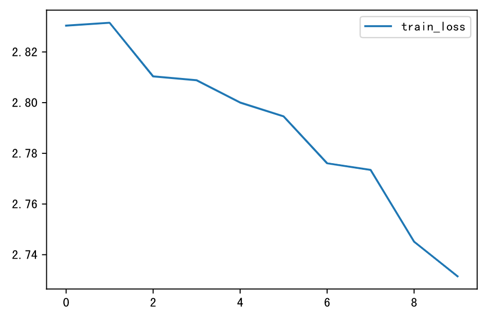
这时验证集上的正确率显著提高了，但是当我们提交测试时，发现得分降低了很多，只有25.38

Loss曲线如下：

如果将weight_decay 恢复为3，学习率的最大值调为0.08，得到测试集正确率达到75.04%

epoch: 1, time cost: 5.766003131866455, avg loss: 2.6178739070892334
epoch: 2, time cost: 5.268301010131836, avg loss: 2.579922676086426
epoch: 3, time cost: 5.208974361419678, avg loss: 2.5794901847839355
epoch: 4, time cost: 5.377782583236694, avg loss: 2.5622220039367676
epoch: 5, time cost: 5.06143856048584, avg loss: 2.5553362369537354
epoch: 6, time cost: 5.280531406402588, avg loss: 2.5241775512695312
epoch: 7, time cost: 5.4181740283966064, avg loss: 2.518286943435669
epoch: 8, time cost: 5.181166410446167, avg loss: 2.493945598602295
epoch: 9, time cost: 5.165584087371826, avg loss: 2.4739253520965576
[WARNING] ME(4323:139631345719104,MainProcess):2021-07-15-19:43:15.811.994 [mindspore/train/model.py:684] CPU cannot support dataset sink mode currently.So the evaluating process will be performed with dataset non-sink mode.
epoch: 10, time cost: 5.15599799156189, avg loss: 2.4562058448791504
validating the model...
{'acc': 0.7504480286738351, 'loss': 2.4718003503737913}

但是得分依然较低：

若改成常数学习率，epoch =10，准确率降为38.84%，并且得分依然不高

如果学习率改为 square decay，其他和最初模型保持一致，并且只训练4个 epoch，防止过拟合，最终结果为：

epoch: 1, time cost: 5.837294340133667, avg loss: 2.589850425720215
epoch: 2, time cost: 5.3242347240448, avg loss: 2.5081369876861572
epoch: 3, time cost: 5.623595476150513, avg loss: 2.4933505058288574
[WARNING] ME(12849:139909491181376,MainProcess):2021-07-15-20:14:56.881.886 [mindspore/train/model.py:684] CPU cannot support dataset sink mode currently.So the evaluating process will be performed with dataset non-sink mode.
epoch: 4, time cost: 5.097643613815308, avg loss: 2.4622089862823486
validating the model...
{'loss': 2.4700695314714984, 'acc': 0.7459677419354839}

且Loss下降很快：

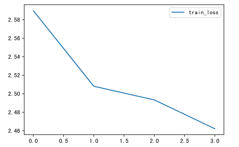
得分为64.62，考虑到每训练一次都要花很多时间，因此综合考虑正确率和得分，我们选择此模型作为最终结果。

模型推理

加载模型Checkpoint进行推理。

使用load_checkpoint接口加载数据时，需要把数据传入给原始网络，而不能传递给带有优化器和损失函数的训练网络。

首先定义图像预处理的函数

def image_process(image):
    """Precess one image per time.一次处理一张图片
    
    Args:
        image: shape (H, W, C)
    """
    mean=[0.485*255, 0.456*255, 0.406*255]
    std=[0.229*255, 0.224*255, 0.225*255]
    image = (np.array(image) - mean) / std # 减均值除以标准差
    image = image.transpose((2,0,1)) #通道，高度，宽度
    img_tensor = Tensor(np.array([image], np.float32))# 转为Tensor
    return img_tensor

def infer_one(network, image_path):
    image = Image.open(image_path).resize((config.image_height, config.image_width))
    logits = network(image_process(image))
    pred = np.argmax(logits.asnumpy(), axis=1)[0]
    print(image_path, inverted[pred])
    return pred

def infer(images):
    backbone = MobileNetV2Backbone()
    head = MobileNetV2Head(input_channel=backbone.out_channels, num_classes=config.num_classes, reduction=config.reduction)
    network = mobilenet_v2(backbone, head)
    print('加载模型路径:',os.path.join(config.save_ckpt_path, CKPT))
    load_checkpoint(os.path.join(config.save_ckpt_path, CKPT), net=network)
    for img in images:
        infer_one(network, img)

下面进行测试集加载

test_images = list()
folder = os.path.join(config.dataset_path, 'val/00_01') # Hats
for img in os.listdir(folder):
    test_images.append(os.path.join(folder, img))

infer(test_images)

导出 MindIR 模型文件

当有了 Checkpoint 文件后，如果想继续基于 MindSpore Lite 在手机端做推理，需要通过网络和 Checkpoint 生成对应的 MindIR 格式模型文件。当前支持基于静态图，且不包含控制流语义的推理网络导出。导出该格式文件的代码如下：

backbone = MobileNetV2Backbone()
# 导出带有Softmax层的模型
head = MobileNetV2Head(input_channel=backbone.out_channels, num_classes=config.num_classes,
                       reduction=config.reduction, activation='Softmax')
network = mobilenet_v2(backbone, head)
load_checkpoint(os.path.join(config.save_ckpt_path, CKPT), net=network)

input = np.random.uniform(0.0, 1.0, size=[1, 3, 224, 224]).astype(np.float32)
export(network, Tensor(input), file_name=config.export_path, file_format='MINDIR')

总结

我们把上述步骤做一下总结

1. 导入相关包
2. 建立垃圾分类数据集标签，以及用于标签映射的字典
3. 指定模型超参数
4. 自定义模型Head部分
5. 训练 Head 部分参数
6. 加载已训练好的网络模型
7. 实现图像预处理
8. 模型预测

预测部分, 对下面这张图像做预测

# 输入图片路径和名称
image_path = './datasets/5fbdf571c06d3433df85ac65-momodel/garbage_26x100/val/00_00/00037.jpg'

# 使用 opencv 读取图片
image = cv2.imread(image_path)

# 打印返回结果
print(predict(image))

预测结果为：Plastic Bottle，说明是可回收垃圾，分类正确。

反思

在调参的过程中，我们发现每调一次参数都要训练一次，在验证集上要运行一遍整个网络，非常耗时，很难在有限时间内得到非常好的模型，单纯靠 “尝试” 调参是很难得到一个很好的模型的，需要一些指导性的方针来指引我们朝正确的方向走下去。因此深度学习目前应该发展借助实验和理论发展出一些好的指导原则，让调参这件事变得不那么玄学。