python机器学习常用模型

python机器学习

算法分类

监督学习

• 定义︰输入数据是由输入特征值和目标值所组成。函数的输出可以是一个连续的值(称为回归)，或是输出是有限个离散值（称作分类)。
• 分类: k-近邻 贝叶斯 决策树 随机森林 逻辑回归
• 回归:线性回归 岭回归

无监督学习

• 定义:输入数据是由输入特征值所组成。
• 聚类: k-means

流程

一，获取数据

当你拿到数据之后，自然而然的你要把数据集进行处理，如果一开始数据就相对于比较嘈杂，如缺失值，或者一些数据不符合我们需要的要求时，就要进行数据处理

二，数据处理

查看是否有明显的异常值，如某些数据点和数据集中的其他值存在明显的差异。通过一维，二维或者三维图形化展示数据是个不错的方法，但是我们得到的数据的特征值都不会低于三个，无法一次图形化展示所有特征。我们可以通过数据的提炼，压缩多维特征到二维或者一维

三，特征工程

其实特征工程也是对数据处理的一种方式，只不过我们会把这些数据处理成更为能被算法进行处理，机器学习的数据集分为 特征值 和 目标值

​ 特征工程包括从原始数据中特征构建、特征提取、特征选择。特征工程做的好能发挥原始数据的最大效力，往往能够使得算法的效果和性能得到显著的提升，有时能使简单的模型的效果比复杂的模型效果好。数据挖掘的大部分时间就花在特征工程上面，是机器学习非常基础而又必备的步骤。数据预处理、数据清洗、筛选显著特征、摒弃非显著特征等等都非常重要。

四，机器学习算法训练

考虑算法是属于监督学习算法还是无监督学习算法。如果使用无监督学习算法，由于不存在目标变量值，故而也不需要训练算法。进而得到模型。

五，模型评估

模型诊断中至关重要的是判断过拟合、欠拟合，常见的方法是绘制学习曲线，交叉验证。通过增加训练的数据量、降低模型复杂度来降低过拟合的风险，提高特征的数量和质量、增加模型复杂来防止欠拟合。诊断后的模型需要进行进一步调优，调优后的新模型需要重新诊断，这是一个反复迭代不断逼近的过程，需要不断的尝试，进而达到最优的状态。通过测试数据，验证模型的有效性，观察误差样本，分析误差产生的原因，往往能使得我们找到提升算法性能的突破点。误差分析主要是分析出误差来源与数据、特征、算法。

数据集

​ scikit-learn : https://scikit-learn.org/stable/datasets

​ uci: http://archive.ics.uci.edu/ml/index.php

​ kaggle: https://www.kaggle.com/datasets

数据集划分

• 训练数据: 用于训练,构建模型
• 测试数据:在模型检验时使用，用于评估模型是否有效

划分比列

训练集	70%	80%	75%
测试集	30%	20%	30%

数据集划分示列

import sklearn.model_selection
from sklearn.datasets import load_iris

def get_data_set():
    iris = load_iris()
    # 参数: x数据集的特征,y数据的特征,测试集的大小(0~1一般默认0.25),随机数种子
    # 返回值: 训练特征值,测试特征值,训练集目标值,测试目标值
    test=sklearn.model_selection.train_test_split(iris.data,iris.target,test_size=0.2,random_state=22)

    pass

特征工程

数据和特征决定了机器学习的上限,模型和算法只是逼近这个上限

特征抽取

• 数据不能直接被算法处理
• 字典特征提取(特征离散化): 数据集类别比较多
• 文本特征提取
• 图像特征提取

one-hot提取字典

from sklearn.feature_extraction import DictVectorizer

# one-hot提取特征字典
def one_hot_feature():
    data = [{
        "city": "成都",
        "temperature": 23
    }, {
        "city": "上海",
        "temperature": 33
    }, {
        "city": "北京",
        "temperature": 16
    }]
    # 字典特征提取,one-hot编码, sparse默认True,返回one hot后的稀疏矩阵
    dic = DictVectorizer(sparse=False)
    one_hot = dic.fit_transform(data)  # 返回one-hot
    print(one_hot)
    print("特征:", dic.get_feature_names(), "\n或者是: ", dic.feature_names_)
    pass

文本特征提取

from sklearn.feature_extraction.text import CountVectorizer
def text_feature():
    data = ["i feel it is good,so i try to eat","i do not feel so good,so i try to sleep"]
    count_vectorize= CountVectorizer()
    word = count_vectorize.fit_transform(data)
    print("特征: ",count_vectorize.get_feature_names())
    print(word.toarray())
    chinese = ["我 今天 感觉 很好 , 所以 我 想 吃 饭",
               "我 今天 感觉 不好, 所以 我 想 睡觉"]
    chinese_count = CountVectorizer()
    words = chinese_count.fit_transform(chinese)
    print("汉子特征: ",chinese_count.get_feature_names())
    print(words.toarray())
    pass

jieba分词

# 精确模式，试图将句子最精确地切开，适合文本分析；
# 全模式，把句子中所有的可以成词的词语都扫描出来, 速度非常快，但是不能解决歧义；
# 搜索引擎模式，在精确模式的基础上，对长词再次切分，提高召回率，适合用于搜索引擎分词。

# 全匹配
seg_list = jieba.cut("今天哪里都没去，在家里睡了一天", cut_all=True)
print(list(seg_list))  # ['今天', '哪里', '都', '没去', '', '', '在家', '家里', '睡', '了', '一天']

# 精确匹配 默认模式
seg_list = jieba.cut("今天哪里都没去，在家里睡了一天", cut_all=False)
print(list(seg_list))  # ['今天', '哪里', '都', '没', '去', '，', '在', '家里', '睡', '了', '一天']

# 搜索匹配
seg_list = jieba.cut_for_search("今天哪里都没去，在家里睡了一天")
print(list(seg_list))  # ['今天', '哪里', '都', '没', '去', '，', '在', '家里', '睡', '了', '一天']

jieba使用方法: https://zhuanlan.zhihu.com/p/100536469

TF-IDF: 评估一字词对于一个文件集或一个语料库中的其中一份文件的重要程度TF: term frequency=改词出现次数/总词数而IDF: inverse document frequency[逆向文档词频] = lg(总文件数目/包含该词语文件数目)

TF-IDF = TF * IDF

from sklearn.feature_extraction.text import TfidfVectorizer
def main():
    xiaoshuo = ["聂凡无语，继续收拾自己的物品，而李财却得瑟的说道“那么拼命又有什么用？还不是白白给我打工。",
                "凡拿起自己整理好的纸箱冷冷的瞪着他说道“别嚣张，你们做的好事迟早会被人知道。说着就往外走去。"]
    tfidf_vectorizer = TfidfVectorizer()
    fenci = []
    for words in xiaoshuo:
        # 迭代器对象可以强转为list
        fenci.append(' '.join(list(jieba.cut(words))))
    feature =  tfidf_vectorizer.fit_transform(fenci)
    print("特征: ", tfidf_vectorizer.get_feature_names())
    print(feature.toarray())
    pass

特征预处理

特征的大小和单位相差较大,或者某些特征的方差相比其他特征要大出几个数量级,容易影响目标结果,其次将数据转换成更适合算法模型的特征数据

无量纲化

• 归一化
• 标准化

最大最小归一化: 缺点: 如果有异常值,离群点,缺失值,都会有很大影响

from sklearn.preprocessing import  MinMaxScaler
# 最大最小归一化
def main():
    data = [[0,2,3,1,5,1,0,0,1,1],
            [1,3,4,1,4,1,3,5,3,2],
            [3 ,0 ,6, 1, 0 ,0 ,1 ,1, 2, 1]]
    print("归一化前: ",data)
    # 指定归一化区间
    min_max_scaler =MinMaxScaler(feature_range=[0,1])
    scale = min_max_scaler.fit_transform(data)
    print("最大最小归一化: ",scale)

    pass

标准化: 标准差用于衡量数据离散程度,如果出现异常点,少量的异常点对于均值的影响不大,方差改变较小,适合大数据比较嘈杂的场景

from sklearn.preprocessing import  StandardScaler
# 标准化[-1,+1]
def main():
    data = [[0, 2, 3, 1, 5, 1, 0, 0, 1, 1],
            [1, 3, 4, 1, 4, 1, 3, 5, 3, 2],
            [3, 0, 6, 1, 0, 0, 1, 1, 2, 1]]
    print("归一化前: ", data)
    stand_scaler = StandardScaler()
    scalse = stand_scaler.fit_transform(data)
    print("标准化后: ",scalse)
    pass

特征降维

• 降低随机变量出现的个数

• 降低特征之间的相关性

• 主成分分析,特征选择

• 特征选择

  • Filter过滤

    • 方差选择

    • 低阶方差特征过滤

    from sklearn.feature_selection import VarianceThreshold
    # 低阶方差特征过滤
    def feature_filter():
        data = [
                [0,0,2,12.8],
                [1,1,3,22.2]]
        # 过滤特征,threshold默认0,小于等于该值的特征方差所对应的特征会被删去
        variance_threshold = VarianceThreshold(threshold=7)
        filter = variance_threshold.fit_transform(data)
        print(filter)
        pass
    

  • Enbeded嵌入式

    • 决策树: 信息熵,信息增益
    • 正则化: L1,L2
    • 深度学习: 卷积

• 主成分分析(PCA)

  from sklearn.decomposition import PCA
  def pca_jiangwei():
      # 可选参数n_components,小数表示降维后保留多少信息,整数表示减少到多少特征
      pca =PCA(n_components=2) # 降到2维
      # 二维特征集
      data = [[1,2,3],[4,5,6]]
      print("降维前:",data)
      result = pca.fit_transform(data)
      print("降维后: ",result)
      pass
  
  

分类与回归算法

K-近邻(KNN)

​ 如果一个样本在空间中的k个最相似(即特征空间中最邻近)的样本中大多数属于某一个类别,则该样本也属于这个类别

样本之间的距离可以使用距离公司计算: 欧氏距离,明可夫斯基距离,曼哈顿距离等

• 优点: 简单,易于理解,无需训练
• 缺点: 懒惰算法,计算量大内存开销大,必须确定k值,k值选择不当分类的精度不能保证,适用于小数据场景

k过小容易受到异常值影响,k过大容易样本不均衡

from sklearn.datasets import load_iris
from sklearn.model_selection import train_test_split
from sklearn.preprocessing import StandardScaler
from sklearn.neighbors import KNeighborsClassifier


# 1. 获取数据集
def get_data():
    return load_iris()


# 2. 划分数据集
def split_data(feature, destination, seed):
    return train_test_split(feature, destination, random_state=seed)


# 3. 特种工程: 标准化
def stand_sample(train, test):
    standd_scaler = StandardScaler()
    return (standd_scaler.fit_transform(train), standd_scaler.transform(test))


# 4. KNN分类学习
def knn(neighbors, x_train, y_train):
    estimator = KNeighborsClassifier(n_neighbors=neighbors)
    estimator.fit(x_train, y_train)
    return estimator


# 5. 模型评估: 直接比对真实值和预测值或者计算准确率
def evaluate_model(model, x_test, y_test):
    predict = model.predict(x_test)
    score = model.score(x_test, y_test)
    return predict, score


def main():
    # 获取鸢尾花数据集
    iris = get_data()
    # 划分鸢尾花的数据集
    x_train, x_test, y_train, y_test = split_data(iris.data, iris.target, 22)
    # 标准化
    x_train, x_test = stand_sample(x_train, x_test)
    model = knn(3, x_train, y_train)
    # 模型评估
    predic, score = evaluate_model(model, x_test, y_test)
    print("预测值: ", predic)
    print("准确率: ", score)
    pass


if __name__ == "__main__":
    main()

朴素贝叶斯

朴素: 特征之间互相独立<=>P(A,B)=P(A)*P(B)

优点:对缺失值不敏感引入了拉普拉斯平滑系数 缺点: 特征属性之间有关联模型会不准确

应用场景:文本分类

from sklearn.model_selection import train_test_split
from sklearn.feature_extraction.text import TfidfVectorizer
from sklearn.datasets import fetch_20newsgroups
from sklearn.naive_bayes import MultinomialNB

# 朴素贝叶斯
def main():
    print("data loading")
    data = fetch_20newsgroups(subset="all")
    print("loading success")
    x_train,x_test,y_train,y_test=train_test_split(data.data,data.target)
    tf_idf = TfidfVectorizer()
    x_train=tf_idf.fit_transform(x_train)
    x_test=tf_idf.transform(x_test)
    estimator = MultinomialNB()
    estimator.fit(x_train,y_train)
    # 模型评估
    predic = estimator.predict(x_test)
    score = estimator.score(x_test,y_test)
    print("预测结果: ",predic)
    print("模型准确率: ",score)
    pass

决策树

高效的决策: 特征的先后顺序很重要,决策树划分依据: 信息熵和信息增益

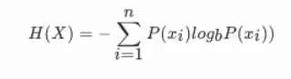
信息就是消除随机不确定性的东西

信息熵

条件熵

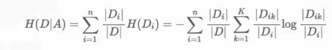
信息增益表示得知特征X的信息不确定性减少的程度使得Y的信息熵减少的程度

from sklearn.model_selection import train_test_split
from sklearn.tree import DecisionTreeClassifier,export_graphviz
from graphviz import Source
def main():
    iris = load_iris()
    x_train,x_test,y_train,y_test=train_test_split(iris.data,iris.target)
    # criterion='gini'默认,也可以选择entropy
    # max_depth树的最大深度,树的深度不能小也不能大,大了会对训练集过度拟合导致实际效果很差
    # random_state随机数种子
    estimator=DecisionTreeClassifier(criterion="entropy")
    estimator.fit(x_train,y_train)
    predic = estimator.predict(x_test)
    score = estimator.score(x_test, y_test)
    print("预测结果: ", predic)
    print("真实值和预测值: ",y_test==predic)
    print("模型准确率: ", score)
    export_graphviz(estimator,out_file="./iris_tree.dot",feature_names=iris.feature_names)

    dot = Source.from_file(filename="./iris_tree.dot",format="pdf")
    # dot.render(filename="iris_tree.pdf",format="pdf")
    dot.render()

逻辑回归–二分类

解决二分类问题

逻辑回归的输入就是线性回归的输出

激活函数:sigmoid

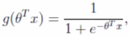
回归的结果输入到sigmoid函数中输出[0,1]

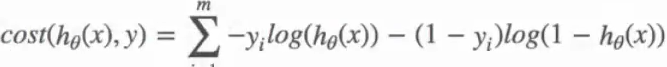
损失函数

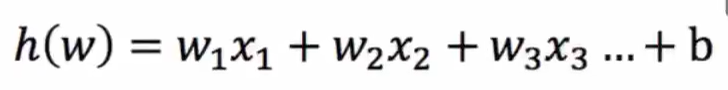
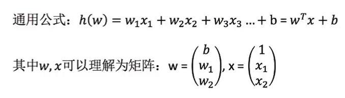
线性回归

目标值: 连续型数据如房价预测,销售额预测

函数关系,多个特征:多元回归

损失函数: 最小二乘法常用的两种优化方法

• 正规方程
• 梯度下降

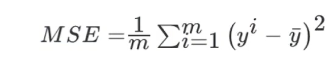
回归性能分析; 均方误差

# 线性回归存在欠拟合和过拟合问题
# 过拟合: 训练集上表现很好,但测试机上不好,一个假设在训练数据上能够获得比其他假设更好的拟合，但是在测试数据集上却不能很好地拟合数据，此时认为这个假设出现了过拟合的现象。(模型过于复杂)
# 欠拟合: 学习的特征太少了,一个假设在训练数据上不能获得更好的拟合，并且在测试数据集上也不能很好地拟合数据，此时认为这个假设出现了欠拟合的现象。(模型过于简单)

# 解决方案
# 欠拟合: 增加特征数量
# 过拟合: 让高次项的项减少--正则化
# L2正则化: 使权重w趋近0,削弱某些特征影响+惩罚项-Ridge岭回归(常用)
# L1正则化: 惩罚项是w的绝对值,导致使w直接为0---LASSO回归

# 线性回归: 正规方程和梯度下降
def main():
    boston = load_boston()
    x_train, x_test, y_train, y_test = train_test_split(boston.data, boston.target)
    print("特征数量: ",boston.data.shape[1])

    stand_scaler = StandardScaler()
    x_train = stand_scaler.fit_transform(x_train)
    x_test = stand_scaler.transform(x_test)
    # 特征有多少个系数就有多少个

    # 正规方差优化,fit_intercept是否计算偏置,偏置表示该函数是否不经过原点,b的值
    line_regress=LinearRegression()
    line_regress.fit(x_train,y_train)
    print("正规方程权重系数: ",line_regress.coef_) # 回归系数
    print("正规方程偏置系数b: ",line_regress.intercept_)# 偏置

    # 梯度下降:loss损失函数 'squared_loss' 最小二乘法,fit_intercept是否计算偏置
    # 学习率learning_rate, 'constant' 常数值,固定步长, 'optimal' ,'invscaling' 步长逐渐减小
    sgd_regress=SGDRegressor()
    sgd_regress.fit(x_train,y_train)
    print("梯度下降权重系数: ",sgd_regress.coef_)  # 回归系数
    print("梯度下降偏置系数b: ",sgd_regress.intercept_)  # 偏置

    # 模型评估,均方误差: 真实值和预测值
    line_predict = line_regress.predict(x_test)
    sgd_predic = sgd_regress.predict(x_test)
    line_err= mean_squared_error(y_test,line_predict)
    sgd_err = mean_squared_error(y_test,sgd_predic)
    print("正规方程均方误差: %f\t梯度下降均方误差: %f" % (line_err,sgd_err))
    pass

岭回归

带L2正则化的线性回归

from sklearn.linear_model import Ridge

# L2正则化,岭回归
def main():
    boston = load_boston()
    x_train, x_test, y_train, y_test = train_test_split(boston.data, boston.target)

    # 正则化力度alpha 0~1或1~10,fit_intercept是否添加偏置
    # solver选择优化方法: dg:梯度下降或sag随机梯度下降
    # normalize标准化
    ridge = Ridge(alpha=1,solver="auto",normalize=True)
    ridge.fit(x_train,y_train)
    print("岭回归权重系数: ", ridge.coef_)  # 回归系数
    print("岭回归偏置系数b: ", ridge.intercept_)  # 偏置
    ridge_predict = ridge.predict(x_test)
    ridge_err = mean_squared_error(y_test, ridge_predict)
    print("岭回归均方误差: ",ridge_err)

    pass

随机森林

包含多个决策树的分类器,其输出的类别是个别树输出类别的众数决定的

• 特征随机: 一次随机选出一个样本重复N次,随机选出m个特征m<<M建立决策树
• 训练集随机: bootstrap随机有放回抽样

适用于大数据,多维有较好的准确率

from sklearn.datasets import load_iris
from sklearn.model_selection import train_test_split,GridSearchCV
from sklearn.ensemble import RandomForestClassifier
from sklearn.preprocessing import StandardScaler
# 随机森林
def main():
    # n_estimators 深林中树的数量
    # criterion分割特征的方法gini默认
    # max_depth 最大深度
    # max_features最大特征
    # bootstrap是否放回抽样默认True
    # min_samples_split节点最少样本数量
    # min_samples_leaf叶子节点最少样本数量
    iris =load_iris()
    x_train, x_test, y_train, y_test = train_test_split(iris.data, iris.target)
    stand_scaler = StandardScaler()
    x_train=stand_scaler.fit_transform(x_train)
    x_test=stand_scaler.transform(x_test)
    rand_forest = RandomForestClassifier()
    param_grid = {
       "n_estimators": [120,200,3000,500,800,1200],
        "max_depth":[5,8,15,25,30],
    }
    estimator = GridSearchCV(rand_forest,param_grid=param_grid,cv=10)
    estimator.fit(x_train,y_train)
    print("最佳参数: ", estimator.best_params_)
    print("最佳结果: ", estimator.best_score_)
    print("最佳估计器: ", estimator.best_estimator_)
    print("交叉验证结果: ", estimator.cv_results_)
    print("准确率: ", estimator.score(x_test, y_test))
    print("预测值: ", estimator.predict(x_test))
    pass

无监督学习

k-means

• 随机设置k个特征空间的点作为聚类中心 k是超参数可以用过网格搜索调优
• 对于其他每个点计算到K个中心的距离，未知的点选择最近的一个聚类中心点作为标记类别
• 接着对着标记的聚类中心之后，重新计算出每个聚类的新中心点(平均值)
• 如果计算得出的新中心点与原中心点一样，那么结束，否则重新进行第二步过程

from sklearn.cluster import KMeans
def main():
    iris = load_iris()
    x_train, x_test, y_train, y_test = train_test_split(iris.data, iris.target)
    #n_clusters聚类中心数量,init初始化方法默认k-means++,labels默认的标记类型可以和真实值比较不是值比较
    estimator = KMeans(n_clusters=3)
    estimator.fit(x_train)
    print("预测: ",estimator.predict(x_test)==y_test)
    
pass

模型选择与调优

交叉验证

使模型评估更加准确

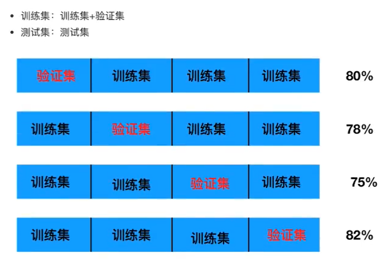
超参数搜索-网格搜索

​ 模型中需要手动指定的参数叫超参数

​ 对模型预设集中超参数,并都采用交叉验证来进行评估最后选择最优参数组合建立模型

def main():
    # 获取鸢尾花数据集
    iris = get_data()
    # 划分鸢尾花的数据集
    x_train, x_test, y_train, y_test = split_data(iris.data, iris.target, 22)
    # 标准化
    x_train, x_test = stand_sample(x_train, x_test)
    model = knn(3, x_train, y_train)
    # 模型评估
    predic, score = evaluate_model(model, x_test, y_test)
    print("预测值: ", predic)
    print("准确率: ", score)

    # 模型调优获取最佳k值
    estimator = KNeighborsClassifier()
    # 准备需要调优的参数
    param_grid = {
        "n_neighbors": range(1,10)
    }
    # cv指定需要几折交叉验证
    grid_search = GridSearchCV(estimator=estimator,param_grid=param_grid,cv=10)
    grid_search.fit(x_train,y_train)
    print("最佳参数: ",grid_search.best_params_)
    print("最佳结果: ",grid_search.best_score_)
    print("最佳估计器: ",grid_search.best_estimator_)
    print("交叉验证结果: ",grid_search.cv_results_)
    print("准确率: ",grid_search.score(x_test,y_test))
    print("预测值: ",grid_search.predict(x_test))
    pass

模型评估

精确率和召回率

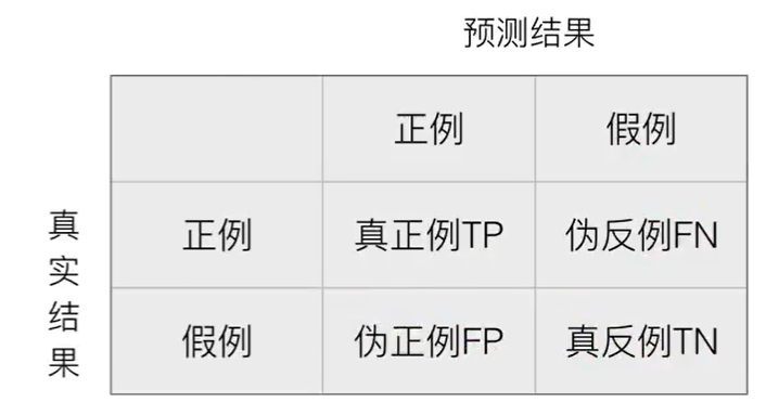
**混淆矩阵 **在分类任务下，预测结果(Predicted Condition)与正确标记(True Condition)之间存在四种不同的组合，构成混淆矩阵(话用于多分类)

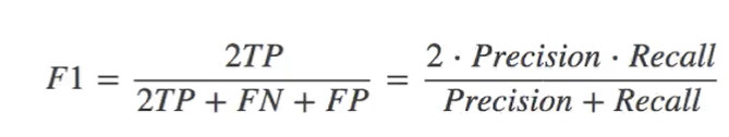
精确率 预测结果为正例样本中真实为正例的比例TP/(TP+FP)

召回率 真实为正例样板中预测结果为正例的比例TP(TP+FN)对正样本的区分能力

F1-score

# 在之前逻辑回归癌症预测中我们可以看到他的精确率,召回率和F1-score
# 参数: 真实值,预测值,labels指定类别对应的数字
report = classification_report(y_test,logistic_predict,labels=[2,4],target_names=["良性","恶性"])
 print(report)
"""
               precision    recall  f1-score   support

          良性       1.00      0.98      0.99       117
          恶性       0.96      1.00      0.98        54

    accuracy                           0.99       171
   macro avg       0.98      0.99      0.99       171
weighted avg       0.99      0.99      0.99       171


"""

ROC曲线和AUC指标

TPR和FPR

• TPR(召回率) = TP / (TP + FN)
• FPR = FP / (FP + TN)

ROC

ROC曲线的横轴就是FPRate，纵轴就是TPRate，当二者相等时，表示的意义则是∶对于不论真实类别是1还是0的样本，分类器预测为1的概率是相等的，此时AUC为0.5

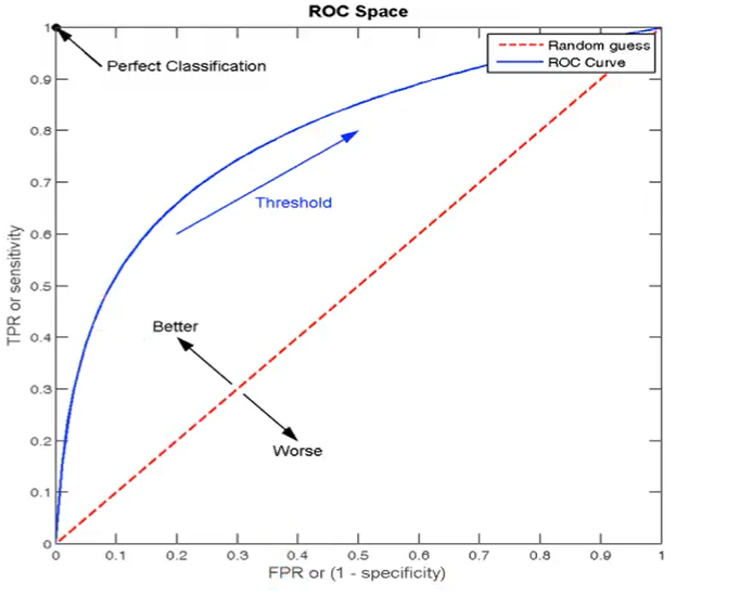
AUC

AUC的概率意义是随机取一对正负样本，正样本得分大于负样本的概率AUC的最小值为0.5，最大值为1，取值越高越好
AUC=1，完美分类器，采用这个预测模型时，不管设定什么阈值都能得出完美预测。绝大多数预测的场合，不存在完美分类器。
0.5<AUC<1，优于随机猜测。这个分类器（模型）妥善设定阈值的话，能有预测价值。

from sklearn.metrics import roc_auc_score

	# ROC 和AUC评估
    # y_true: 每个样本的真实类别，必须为0(反例), 1(正例)标记
    # y_score: 预测得分，可以是正类的估计概率、置信值或者分类器方法的返回值
    y_true = np.where(y_test>3,1,0)
    roc_auc = roc_auc_score(y_true,y_score=logistic_predict)
    print("roc-auc: ", roc_auc)

轮廓系数

高类聚,低耦合评判聚类算法

轮廓系数:注:对于每个点i为已聚类数据中的样本，b_i为i到其它族群的所有样本的距离最小值,a_i为i到本身簇的距离平均值。最终计算出所有的样本点的轮廓系数平均值

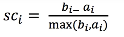
轮廓系数范围[-1,1],越接近1模型越好,越接近-1模型月初

def main():
    iris = load_iris()
    x_train, x_test, y_train, y_test = train_test_split(iris.data, iris.target)

    #n_clusters聚类中心数量,init初始化方法默认k-means++,labels默认的标记类型可以和真实值比较不是值比较
    estimator = KMeans(n_clusters=3)
    estimator.fit(x_train)
    y_predict = estimator.predict(x_test)
    print("预测: ",y_predict==y_test)
    # 轮廓系数
    score = silhouette_score(x_test,y_predict)
    print("轮廓系数: ",score)
pass

模型保存和加载

import joblib
def main():
    iris = load_iris()
    x_train, x_test, y_train, y_test = train_test_split(iris.data, iris.target)
    estimator = DecisionTreeClassifier(criterion="entropy")
    estimator.fit(x_train, y_train)
    predic = estimator.predict(x_test)
    score = estimator.score(x_test, y_test)
    print("预测结果: ", predic)
    print("真实值和预测值: ", y_test == predic)
    print("保存模型")
    joblib.dump(estimator,"./iris_tree.pkl")
    print("加载模型")
    estimator = joblib.load("./iris_tree.pkl")
    predic = estimator.predict(x_test)
    print("预测结果: ", predic)
    print("真实值和预测值: ", y_test == predic)
    pass