【数值分析×机器学习】以SVD的分解形式进行深度神经网络的训练（逐渐熟练）

• 英文标题：Learning Low-rank Deep Neural Networks via Singular Vector Orthogonality Regularization and Singular Value Sparsification
• 中文标题：学习低秩深度神经网络通过奇异向量正交正则化与奇异值稀疏化
• 论文下载链接：arxiv@2004.09031v1
• 论文项目地址：暂时没找到

序言

写proposal前的最后一篇paper，这部分内容还是很有意思的，很开拓思路，值得深究。

其实一共是看了四篇，前两篇的笔注：

1. 【数值分析×机器学习】稀疏矩阵向量乘（SpMV）的运行时间预测
2. 【数值分析×机器学习】使用CNN进行雅可比预条件子的生成

第三篇因为太短我放在本文最后做个收尾，这个第四篇很有东西，可惜没能找到项目地址，不知道具体代码实现情况如何。

总之利用这些数值分析的方法来优化DNNs确实是一条很有趣的道路。

$\text{Prescript}$

好天气碰上休假，手环刚到，去试个半马，晚上开写proposal，到底还是这样平淡的生活比较适合我，其实现在一个人待在空屋里还是会有点躁动，从俭入奢易，由奢入俭难，体验过两个人的生活，总是就很难一下子再习惯孤独，不过倒也无妨，这种日子我也不是第一次过了，人总归还是要做回自己才行。

应当期待好的事情终会发生。

---

---

摘要 Abstract

• 深度神经网络（deep neural networks，下简称为DNNs）需要大量的算力成本，所以为了使得DNNs能够在移动设备上使用，一系列诸如因子化（factorization）的方法已经得到了广泛的应用。

  所谓因子化即将DNNs模型中网络层的权重矩阵分解为若干低秩矩阵的乘积，然而在模型训练过程中往往很难衡量矩阵的秩。

  因此前人的工作主要是在模型训练的每一步中引入间接近似（implicit approximations）或高成本的奇异值分解（singular），前者往往会导致较高的训练损失，后者则运行效率很低。

• 本文结合两种方法的优势，提出奇异值分解训练（SVD training）的方法概念，这是目前第一种无需在训练中采用SVD即可直接取得低秩DNNs的方法。

  SVD训练首先将每个网络层的权重矩阵分解成满秩SVD的形式，然后直接就可以在分解得到的一系列权重矩阵上进行训练。

  • 备注：满秩SVD应该就是thin SVD的意思，即$A=UD{V}^{\top }$，其中$D={\mathbb{R}}^{\text{rank}(A)\times \text{rank}(A)}$

    修正：满秩SVD就是不省略任何奇异值的分解，因为$A={\sum }_{i=1}^{\text{rank}(A)}{\sigma }_i{u}_i{v}_i^{\top }$，这就是满秩分解，如果求和项只取到前$k$项，即只取前$k$大的奇异值，就是近似分解。

• 本文在奇异值向量中加入正则化（regularization），从而确保SVD的形式有效（valid form），且可以避免梯度消失或梯度爆炸（gradient vanishing/exploding）。低秩可以通过对每个网络层应用稀疏导出正则器（sparsity-inducing regularizers）来促成。最后会采用奇异值剪枝（Singular value pruning）来直接得到一个低秩模型。

• 本文经验性地（empirically）证明SVD训练可以显著地减小DNNs网络的秩，并且与目前常规的因子化方法以及先进的过滤剪枝方法（filter pruning methods）可以在相同的精确度下大大减少算力开销。

---

1 引入 Introduction

• DNNs的高性能的背后是极高的内存占用与计算负载：

  如$\text{ResNet-50}$模型大约需要$\text{4G}$次浮点运算（floating-point operations，下简称为FLOPs）来分类一张$224\times 224$像素的图片。这是制约DNNs模型在移动智能设备上运行的主要原因。

• DNNs模型的压缩技术的相关研究：

  1. 参考文献$[7,21,38]$：元素级别的剪枝（element-wise pruning）；
  2. 参考文献$[33,25,20]$：结构化剪枝（structural pruning）；
  3. 参考文献$[23,31]$：离散化（quantization）；这个可以参考二进制的嵌入，应该算是一种离散化方法。
  4. 参考文献$[15,39,36,35]$：因子化（factorization）；

  方法$1$和$3$可以有效地减少模型的内存占用，但是需要特殊的硬件来实现高效的计算。

  方法$2$是通过移除冗余的filters和channels来减少计算负载，但是这种方法可能会导致移除后相邻网络层的输出输入无法衔接，因此是需要一些调整技巧的。

  方法$4$即使用若干低秩矩阵的乘积来近似权重矩阵，这种方法天然地可以保持网络层输入输出的维度。

  • 备注：关于结构化剪枝可以参考文章，综合写了多篇与结构化剪枝相关的问题，其实就是丢掉一些冗余的网络层。

• 权重矩阵近似的相关研究：

  1. 参考文献$[15,39,26,4,19]$：使用预训练的DNNs模型生成低秩矩阵的乘积来近似权重矩阵，但是这些方法基变通过了后微调，仍然会严重损害原模型的性能。

  2. 参考文献$[34,20]$：调整filters的方向（directions）来间接地给权重矩阵降秩，但是训练地困难性以及以及矩阵秩的隐含性（implicitness）使得这些方法很难取得一个较高的压缩率。

  3. 参考文献$[1,35]$：使用矩阵的核模（nuclear norm）来作为衡量矩阵秩的依据，但是优化矩阵的核模的效率是很低。

     • 备注：关于矩阵的核模，定义为$\Vert X{\Vert }_{\ast }=\text{tr}\left(\sqrt{X^{\top }X}\right)={\sum }_i^{\text{X}}|{\sigma }_i|$，即所有奇异值绝对值的加和。

• 本文的研究：

  1. 本文旨在直接在模型训练过程中获得一个低秩DNNs模型，而无需在训练的每一步采用SVD；

  2. 本文提出SVD训练的方法，通过训练得到每一层的权重矩阵的满秩SVD形式，权重矩阵分解为左奇异向量，奇异值和右奇异向量，然后训练的目标就是这些分解得到的变量。

     • 备注：这里的意思应该是说神经网络的训练是基于这些分解得到的矩阵进行的，而不是直接用权重矩阵介入网络的训练，其实这件事情应该是可行的，虽然笔者还没有看到下面，但是本身来说你可以理解为是把一个网络层分解成三个低秩的网络层，这个其实并不影响神经网络的反向传播，然后在定义损失函数的时候把这些网络层和秩相关的数字给加进去就可以了。

  3. 进一步地，本文在SVD训练中提出两种技术用于在保持高性能，且可以导出低秩性：

     • 奇异向量正交正则化（singular vector orthogonality regularization）：可以使得奇异向量矩阵在训练过程中尽可能地接近正交矩阵（unitary），这样可以缓和模型训练中梯度消失与梯度爆炸的问题，且可以确保最后得到的SVD形式是合理的，可以用于降秩。

     • 奇异值稀疏化（singular value sparisification）：在模型训练中将稀疏导出正则器（sparsity-inducing regularizers）应用在奇异值上，从而得到低秩矩阵。最终低秩模型是通过奇异值剪枝（singular value pruning）。

  4. 本文对每一种技术都进行了评估（通过消融实验），结果表明本文在提出的方法在各种任务与模型架构上都击败了先进的因子化以及结构化剪枝方法。

  5. 就我们所知，这是第一个用来对每个DNNs网络层在训练过程中（无需进行矩阵分解）对最优秩进行搜索的方法。

---

2 低秩深度神经网络的相关工作 Related Works on Low-rank DNNs

使用低秩矩阵的乘积来近似权重矩阵是压缩DNNs模型的一个非常直接的想法，前人的工作主要集中在设计矩阵或张量分解的架构。

1. 参考文献$[19]$：对四维卷积核张量的分解研究。如张量秩分解（CPD），可以将四维卷积核直接分解为四个低秩的卷积层。

• 备注：CPD这个词我第一次是在RE2RNN那篇paper里碰到的，在那篇博客里有关于CPD的详细说明，对于三维张量的CPD应该是会分解成三个二维矩阵，但是对于四维张量的话，分解得到的矩阵数量可能会非常多。

2. 参考文献$[29]$：上述张量分解技术会使得模型中网络层的数量变得非常多，因此很难通过微调得到很好的性能，尤其是对又大又深的模型进行分解时。

3. 参考文献$[39]$：因此后续有学者研究如何将一个四维张量重构（reshape）成一个二维矩阵，然后再使用针对二维矩阵的分解方法（如SVD），最终再把分解得到的合成结果再重构回四维张量，得到两个连续的网络层（consecutive layers）。在这篇参考文献中，作者提出channel级别的分解（channel-wise decomposition），使用的是SVD来分解卷积层（卷积核的大小维$w\times h$）得到两个连续的网络层（大小分别为$w\times h$和$1\times 1$），然后通过考察channel级别上的冗余（redundancy），如那些带有较小奇异值的channel就可以被移除。

   • 备注：channel在卷积层中一般指图片的通道数，如RGB格式的图片通道数为$3$，RGBA的通道数则为$4$。filter在卷积层中就是卷积核的意思，如果channel数大于$1$，则就是channel数个卷积核的整体称为filter。

4. 参考文献$[15]$：作者类似地也提出一种将卷积层分解成两个连续的网络层的方法，且这两个连续的网络层之间的channel数更少，然后再进一步地利用空间级别的（spatial-wise）冗余来减少卷积核的大小，最终得到的分解网络层的大小分别是$1\times h$和$w\times 1$。这里作者提到说可以在得到满秩分解后手动地选取若干较大的奇异值得到最终的近似结果，但是这样无可避免地会导致较高地精确度损失，虽然压缩率会提升。

一些其他研究着重于如何在降秩的前提下，还能保证模型的精确度损失不会太大。

5. 参考文献$[34]$：采用attractive force正则器来提高某一网络层中不同filters的相关性（correlation）。

6. 参考文献$[5]$：采用centripetal SGD，将多个filters移向一套聚合中心。（不懂，要看原文才行）

   这两种方法都可以减少权重矩阵的秩，而无需在训练中进行低秩分解。

   但是在这两种方法中矩阵的秩都是间接表示的（不知道是什么间接表示），因此正则化的效用的很弱的，可能会导致模型性能骤降（因为追求高处理速度）

7. 参考文献$[1,35]$：使用核模（即所有奇异值绝对值的加和）来表示矩阵的秩，这些方法需要进行SVD，算法复杂度为$\mathcal{O}(n^3)$，且梯度下降法不能直接作用在SVD上（参考文献$[6]$），因此是不太行得通的。

8. 参考文献$[29]$：提出直接训练神经网络得到低秩分解形式，从而直接获得一个低秩网络，无需在训练中的每一步进行高成本的矩阵分解。

9. 参考文献$[14]$：解决矩阵分解后的梯度消失与梯度爆炸问题。

   但是这些方法需要在训练前先对每个网络层的秩进行设定，而手动选择低秩可能无法取得最优的压缩，且训练低秩模型意味着模型优化非常困难，因为低秩意味着模型的容量（capacity）是很低的。

---

3 提出的方法 Proposed Method

• 本文结合分解训练（decomposed）与训练低秩（trained low-rank）两种思想，如$\text{Figure 1}$所示：

  

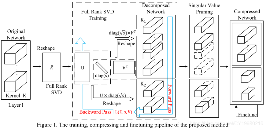
  模型首先通过满秩SVD训练的分解后形式进行训练，然后进行奇异值剪枝（用于降秩），最后再进行进一步的微调（提升精确度）。

• 在Section 3.1中将会说明本文的模型将以空间级（spatial-wise，参考文献$[15]$）或者管道级（channel-wise，参考文献$[39]$）分解的形式进行训练，这样可以避开耗时的SVD。

  与参考文献$[29]$提出的训练步骤不同，本文将对模型进行满秩分解，以确保模型的容量（capacity）。

  在SVD训练中，本文对奇异向量矩阵采用正交正则化（orthogonality regularization），每一层对奇异值采用稀疏导出正则器（sparsity-inducing regularizers），细节分别见Section 3.2&3.3。

  在Section 3.4中论述SVD训练的目标函数以及总体模型的压缩管道（compression pipeline），目的是取得最好的压缩效果。

3.1 深度神经网络的SVD训练 SVD training of deep neural networks

• 本文提出通过神经网络的SVD形式来训练神经网络，其中每个网络层都被分解为两个连续的层（它们之间不存在额外的运算），具体而言对于权重矩阵$W\in {\mathbb{R}}^{m\times n}$，可以分解为$U\in {\mathbb{R}}^{m\times r},V\in {\mathbb{R}}^{n\times r},s\in {\mathbb{R}}^s$三部分，其中$U$与$V$是正交矩阵，在满秩的情况下，即$r=\min (m,n)$，$W$可以精确地被重构成$W=U\text{diag}(s)V^{\top }$。

• 对于神经网络而言，这相当于是将权重矩阵$W$分解为两个连续的层：$W_1=U\text{diag}(\sqrt{s})$与$W_2=\text{diag}(\sqrt{s})V^{\top }$

• 对于卷积层而言，卷积核$\mathcal{K}\in {\mathbb{R}}^{n\times c\times w\times h}$可以表示为一个四维张量，其中$n,c,w,h$分别代表过滤器（filters）的数量，输入管道（channels）的数量，过滤器的宽和高，本文只要使用空间级（spatial-wise，参考文献$[15]$）或者管道级（channel-wise，参考文献$[39]$）分解的方法来对卷积层进行分解（因为前人用下来效果很好）：

  1. 首先将$\mathcal{K}$重构（reshape）成二维矩阵$\hat{K}\in {\mathbb{R}}^{n\times cwh}$；

  2. 然后$\hat{K}$通过SVD得到$U\in {\mathbb{R}}^{n\times r},V\in {\mathbb{R}}^{cwh\times r},s\in {\mathbb{R}}^r$，其中$U$和$V$是正交矩阵，$r=\min (n,cwh)$；

  3. 此时原始的卷积测出那个被分解为两个连续的子卷积层：${\mathcal{K}}_1\in {\mathbb{R}}^{r\times c\times w\times h}$（从$\text{diag}(\sqrt{s})V^{\top }$重构回）与${\mathcal{K}}_2\in {\mathbb{R}}^{n\times r\times 1\times 1}$（从$U\text{diag}(\sqrt{s}))$重构回）；

• 接下来就是空间级的分解，过程与上面管道级的分解类似：

  1. 首先将$\mathcal{K}$重构（reshape）成二维矩阵$\hat{K}\in {\mathbb{R}}^{nw\times ch}$；

  2. 然后就可以得到分解后的矩阵${\mathcal{K}}_1\in {\mathbb{R}}^{nw\times r}$与${\mathcal{K}}_2\in {\mathbb{R}}^{n\times r\times w\times 1}$；

  这种满秩分解模型往往可以取得与原模型相似的精确度。

• 在SVD训练中，每一层使用的都是经过分解后得到的变量，即$U,s,V$，而非原始卷积核$K$或是权重矩阵$W$。前向传递（forward pass）是通过将$U,s,V$转换成两个连续的网络层（如上文所述），反向传播（back propagation）与优化都直接作用在$U,s,V$上。这样我们就可以获得$s$而无需在训练的每一步都执行SVD

• 注意$U,V$需要变成正交矩阵，以确保可以执行低秩近似（low rank approximation），即移除掉较小的奇异值，但是正交的性质不是很容易能够在训练中得到，因此本文加入了一个正交正则化（orthogonality regularization）作用在矩阵$U$和$V$上来处理这个问题（详见Section 3.2）。此外降秩是通过在$s$上应用稀疏导出正则器（sparsity-inducing regularizers）得到的（详见Section 3.2）。

3.2 奇异值向量的正交正则器 Singular vectors orthogonality regularizer

• 为了使得$U,V$尽可能地满足正交的性质，使用下面的正交正则化的损失函数：
  $$L_o(U,V)=\frac{1}{r^2}\left({\Vert U^{\top }U-I\Vert }_F^2-{\Vert V^{\top }V-I\Vert }_F^2\right)\text{\hspace{1em}(1)}$$
  其中$\Vert \cdot {\Vert }_F$是$F$范数，$r$是矩阵$U$和$V$的秩，注意根据定义$U$和$V$的秩在训练中一定是相等的。因此只需要在最终的目标函数中添加式$(1)$的约束即可达到训练出正交矩阵的效果。

• 注意到加入式$(1)$这种损失函数的另一个好处是可以削弱梯度爆炸或梯度消失的问题，因为此时$U$与$V$的列向量的二模接近$1$，因此就不太可能发生梯度爆炸或梯度消失的问题。

3.3 奇异值稀疏导出正则器 Singular values sparsity-inducing regularizer

• 在奇异向量矩阵已经接近正交的前提下，减小分解网络的秩等价于使得每个网络层奇异值向量$s$尽可能的稀疏。虽然可以用零范数（即统计非零元的数量）来表示稀疏度，但是零范数不太容易通过梯度方法进行优化，因此本文启发于参考文献$[21,33]$中的DNNs剪枝，使用一种可微的（differentiable）稀疏导出正则器来使得$s$中更多的元素接近零，然后再使用后剪枝的方法使得奇异值向量尽可能稀疏。

• 一般使用一范数（即所有元素的绝对值之和）来替代零范数，一范数广泛应用于如特征选取（feature selecting）与DNNs剪枝的问题中，因为一范数是凸的（其实就是个线性函数，${\sum }_i|s_i|$），而且奇异值向量$s$的一模正则项等价于是在正则化原始权重矩阵的核模（nuclear norm），这是一种非常经典的用于近似矩阵秩的方法。

  • 备注：这里插个题外话，像一些任务的目标函数是最小化某个矩阵的秩，所以目标函数会是一个矩阵的核模（nuclear norm），但是核模实在是太难优化，所以会转换为零模，正如上面所说，零模还是很难优化，所以要转换为一模。

    一个非常经典的例子就是图像复原，比如给定一张像素图，从中去除掉$80\%$的像素点，问题是如何恢复这张图片，方法就是最小化这个图片所对应矩阵的核模，当然正如上面所说其实最终是转换为一模，有兴趣的可以试试，这种复原方法还真的挺有效果。

• 但是问题在于一模是会随原向量的放缩而等比例放缩的，即$\Vert \alpha W{\Vert }_1=|\alpha |\Vert W{\Vert }_1$，因此$s$的一模会随着奇异值的大小减小而明显减小，前人也设计过不变长的（scale-invariant）模数定义：（Hoyer正则器，参考文献$[16]$）
  $$L^H(s)=\frac{\Vert s{\Vert }_1}{\Vert s{\Vert }_2}=\frac{{\sum }_i|s_i|}{\sqrt{{\sum }_i{s}_i^2}}\text{\hspace{1em}(2)}$$
  即为一模与二模的比值，显然$L^H$可微且不变长，这样就可以使得奇异值向量$s$尽可能的稀疏了。

  在Section 4.3种有关于$L^H$与一范数的性能对比。

3.4 总体目标和训练步骤 Overall objective and training procedure

• 最终分解训练（decomposed training）的目标函数定义如下：
  $$L(U,s,V)=L_T\left(\text{diag}\left(\sqrt{|s|}\right)V^{\top },U\text{diag}\left(\sqrt{|s|}\right)\right)+{\lambda }_o\sum _{l=1}^D{L}_o(U_l,V_l)+{\lambda }_s\sum _{l=1}^D{L}_s(s_l)\text{\hspace{1em}(3)}$$
  其中：

  1. $L_T$是在分解的网络层上的训练损失；
  2. $L_o$是式$(1)$种的正交损失；
  3. $U_l,V_l,s_l$是网络层$l$的奇异向量矩阵与奇异值向量，$D$即为总的网络层数；
  4. $L_s$是稀疏导出正则化的损失，这里对比了$L_s=L^H$以及$L_s=L^1$的性能；
  5. ${\lambda }_o$与${\lambda }_s$是衰减参数（decay parameters），其中${\lambda }_o$可以选成一个很大的正数，以确保正交性，${\lambda }_s$则可以在精确度与FLOPs间进行权衡以得到一个低秩模型；

• 如$\text{Figure 1}$所示，低秩分解网络是通过三阶段操作完成的：

  1. 满秩SVD训练
  2. 奇异值剪枝
  3. 低秩微调

  首先我们训练一个满秩分解网络（使用式$(3)$种的目标函数），这样是可以很容易地得到一个与原模型具有相近性能的分解模型的，因为在满秩分解中矩阵信息是没有任何损失的。

  通过稀疏导出正则器，大多数的奇异值会减小到零。

  启发于参考文献$[35]$的工作，本文使用一种基于能量（energy）的阈值对奇异值进行剪枝，即对于每个网络层，我们寻找一个集合$\mathbb{K}$，其中包含最大数量的奇异值，满足：
  $$\sum _{j\in \mathbb{K}}{s}_j^2\le e\sum _{i=1}^r{s}_i^2\text{\hspace{1em}(4)}$$
  其中$e\in [0,1]$是一个预先定义好的能量阈值，若$e$足够小，则集合$\mathbb{K}$中的奇异值可以安全地被移除掉，而不太影响模型性能，奇异值剪枝的过程即为降秩的过程。

  举个栗子，针对卷积核$\mathcal{K}\in {\mathbb{R}}^{n\times c\times w\times h}$，如果我们可以将分解得到的网络层的秩减小到$r$，那么卷积层FLOPs的运算次数就会减少$\frac{(n+chw)r}{nchw}$或$\frac{(nw+ch)r}{nchw}$（使用空间级或管道级的分解），实验结果现实低秩模型可以通过将${\lambda }_s$设置得接近零来进一步提升模型性能。

---

4 实验结果 Experiment Results

本文在$\text{CIFAR-10}$数据集（参考文献$[17]$）上的$\mathrm{R}\mathrm{e}\mathrm{s}\mathrm{N}\mathrm{e}\mathrm{t}$模型（参考文献$[9]$）进行消融研究，然后将本文提出的分解训练方法应用在各种不同的DNNs模型上（在$\text{CIFAR-10}$数据集和$\text{ImageNet ILSVARC-2012}$数据集上训练，参考文献$[28]$），附录$\mathrm{A}$中描述了模型训练的超参数，为了在精确度与FLOPs间取得折衷，还测试了很多其他的超参数。

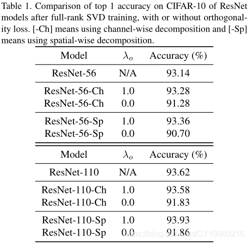
4.1 正交约束的重要性 Importance of the orthogonal constraints

• 如$\text{Table 1}$所示：其实就是测试目标函数有$L_o$项与没有$L_o$项下的一个对比情况，显然有$L_o$项的情况下精确度要高一些，虽然高得也不是太多。

  

4.2 分解方法的比较 Comparison of decomposition methods

• 如$\text{Figure 2}$所示，对空间级与管道级（见Section 3.1详述）得分解方法进行了对比（基于FLOPs与精确度的权衡）：

  

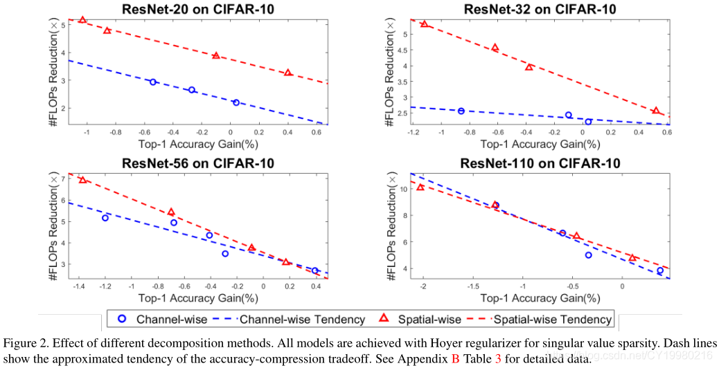
  结论是：

  … spatial-wise decomposition can utilize both spatial-wise redundancy and channel-wise redundancy, while the channel-wise decomposition utilizes channel-wise redundancy only.

  即空间级分解方法的效果应该是要好一点的，因为目前来说DNNs模型倾向于有更多的channel，于是就会导致较为显著的管道级冗余。

4.3 稀疏导出正则器的比较 Comparison of sparsity-inducing regularizers

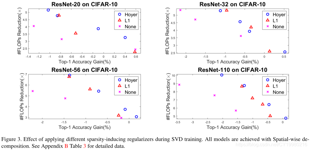
• 如$\text{Figure 3}$所示，就是在比较$L^1$与$L^H$两个正则项的效果（基于空间级分解的方法，因为上一节已经说明这种分解方法更好）：

  

  结论：

  1. The tradeoff tendency of the $L^1$ regularizer constantly demonstrates a larger slope than that of the Hoyer regularizer.
  2. 低精确度损失的情况下，$L^H$可以取得更高的压缩率。
  3. 若容许较高的精确度损失，则$L^1$可以取得更高的压缩率。
  4. 总之对奇异值进行稀疏导出正祖华很重要，因为训练过程中权重矩阵并不会自然而然地趋向于低秩。

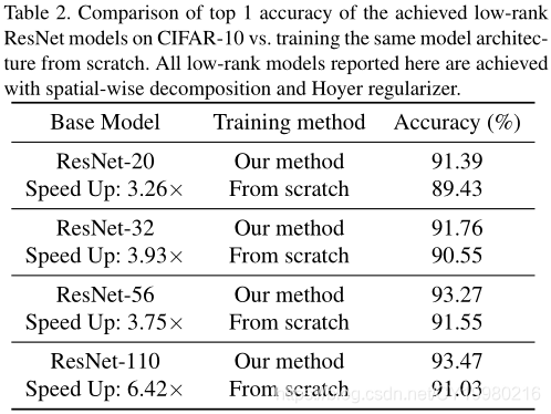
4.4 总体训练步骤的影响 Effectiveness of the overall training procedure

• 本节是针对$\text{Figure 1}$中提出的：

  1. 满秩SVD训练
  2. 奇异值剪枝
  3. 低秩微调

  的框架进行的分析，如$\text{Table 2}$所示，总之就是本文的方法很好呗，看起来确实是这样的：

  

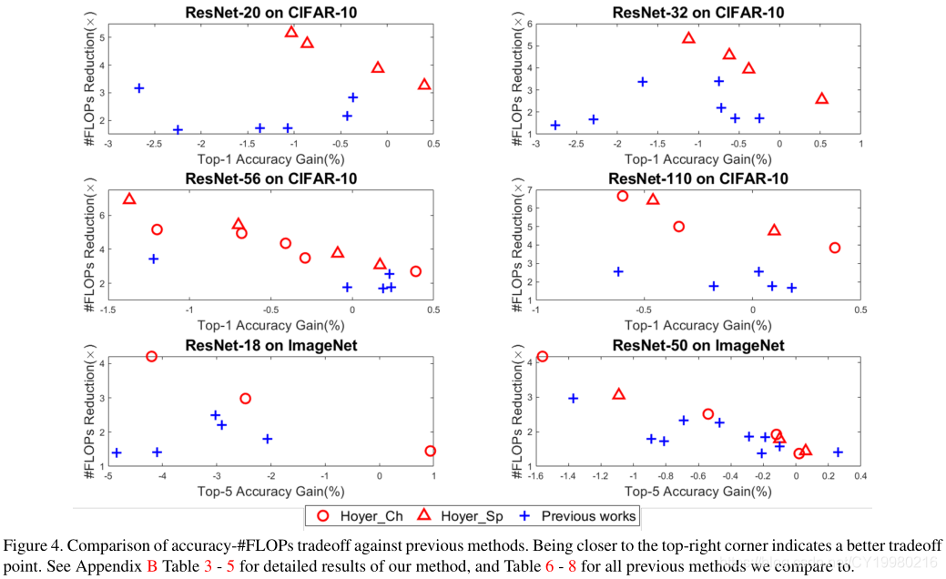
4.5 与前人工作的比较 Comparing with previous works

• 本文将提出的方法框架应用在$\text{ResNet-20,ResNet-32,ResNet-56,ResNet-110}$上（基于$\text{CIFAR-10}$模型），然后与参考文献$[15,39,35,5]$（低秩分解方法）以及参考文献$[37,10,20]$的过滤剪枝方法进行了对比，详细结果见$\text{Figure 4}$：

  

---

5 总结 Conclusion

略，无重要内容。一些实验的细节内容在附录中，这里不再展示，图片太长了。

致谢 Acknowledgments

This work was supported in part by NSF-1910299, NSF-1822085, DOE DE-SC0018064, and NSF IUCRC-1725456, as well as supports from Ergomotion, Inc.

---

参考文献

[01]  Jose M Alvarez and Mathieu Salzmann. Compression-aware training of deep networks. In Advances in Neural Information Processing Systems, pages 856–867, 2017. 2 
[02]  Alfredo Canziani, Adam Paszke, and Eugenio Culurciello. An analysis of deep neural network models for practical applications. arXiv preprint arXiv:1605.07678, 2016. 1 
[03]  Liang-Chieh Chen, George Papandreou, Iasonas Kokkinos, Kevin Murphy, and Alan L Yuille. Deeplab: Semantic image segmentation with deep convolutional nets, atrous convolution, and fully connected crfs. IEEE transactions on pattern analysis and machine intelligence, 40(4):834–848, 2017. 1 
[04] Emily L Denton, Wojciech Zaremba, Joan Bruna, Yann LeCun, and Rob Fergus. Exploiting linear structure within convolutional networks for efficient evaluation. In Advances in neural information processing systems, pages 1269–1277, 2014. 1, 2 
[05]  Xiaohan Ding, Guiguang Ding, Yuchen Guo, and Jungong Han. Centripetal sgd for pruning very deep convolutional networks with complicated structure. In Proceedings of the IEEE Conference on Computer Vision and Pattern Recognition, pages 4943–4953, 2019. 1, 2, 6, 11 
[06]  M Giles. An extended collection of matrix derivative results for forward and reverse mode algorithmic differentiation. an extended version of a paper that appeared in the proceedings of ad2008. In the 5th International Conference on Automatic Differentiation, 2008. 2 
[07]  Song Han, Jeff Pool, John Tran, and William Dally. Learning both weights and connections for efficient neural network. In Advances in neural information processing systems, pages 1135–1143, 2015. 1 
[08] Kaiming He, Georgia Gkioxari, Piotr Doll´ar, and Ross Girshick. Mask r-cnn. In Proceedings of the IEEE international conference on computer vision, pages 2961–2969, 2017. 1 
[09]  Kaiming He, Xiangyu Zhang, Shaoqing Ren, and Jian Sun. Deep residual learning for image recognition. In Proceedings of the IEEE conference on computer vision and pattern recognition, pages 770–778, 2016. 1, 5 
[10]  Yang He, Guoliang Kang, Xuanyi Dong, Yanwei Fu, and Yi Yang. Soft filter pruning for accelerating deep convolutional neural networks. arXiv preprint arXiv:1808.06866, 2018. 6, 11 
[11]  Patrik O Hoyer. Non-negative matrix factorization with sparseness constraints. Journal of machine learning research, 5(Nov):1457–1469, 2004. 4 
[12] Jie Hu, Li Shen, and Gang Sun. Squeeze-and-excitation networks. In Proceedings of the IEEE conference on computer vision and pattern recognition, pages 7132–7141, 2018. 1 
[13] Gao Huang, Zhuang Liu, Laurens Van Der Maaten, and Kilian Q Weinberger. Densely connected convolutional networks. In Proceedings of the IEEE conference on computer vision and pattern recognition, pages 4700–4708, 2017. 1 
[14]  Sergey Ioffe and Christian Szegedy. Batch normalization: Accelerating deep network training by reducing internal covariate shift. arXiv preprint arXiv:1502.03167, 2015. 2 
[15]  Max Jaderberg, Andrea Vedaldi, and Andrew Zisserman. Speeding up convolutional neural networks with low rank expansions. arXiv preprint arXiv:1405.3866, 2014. 1, 2, 3, 6, 11 
[16]  Dilip Krishnan, Terence Tay, and Rob Fergus. Blind deconvolution using a normalized sparsity measure. In CVPR 2011, pages 233–240. IEEE, 2011. 4 
[17]  Alex Krizhevsky and Geoffrey Hinton. Learning multiple layers of features from tiny images. Technical report, Citeseer, 2009. 5, 11 
[18]  Alex Krizhevsky, Ilya Sutskever, and Geoffrey E Hinton. Imagenet classification with deep convolutional neural networks. In Advances in neural information processing systems, pages 1097–1105, 2012. 1 
[19] Vadim Lebedev, Yaroslav Ganin, Maksim Rakhuba, Ivan Oseledets, and Victor Lempitsky. Speeding-up convolutional neural networks using fine-tuned cp-decomposition. arXiv preprint arXiv:1412.6553, 2014. 1, 2 
[20]  Tuanhui Li, Baoyuan Wu, Yujiu Yang, Yanbo Fan, Yong Zhang, and Wei Liu. Compressing convolutional neural networks via factorized convolutional filters. In Proceedings of the IEEE Conference on Computer Vision and Pattern Recognition, pages 3977–3986, 2019. 1, 2, 6, 11 
[21]  Baoyuan Liu, Min Wang, Hassan Foroosh, Marshall Tappen, and Marianna Pensky. Sparse convolutional neural networks. In Proceedings of the IEEE Conference on Computer Vision and Pattern Recognition, pages 806–814, 2015. 1, 4 
[22]  Wei Liu, Dragomir Anguelov, Dumitru Erhan, Christian Szegedy, Scott Reed, Cheng-Yang Fu, and Alexander C Berg. Ssd: Single shot multibox detector. In European conference on computer vision, pages 21–37. Springer, 2016. 1 
[23]  Zechun Liu, Baoyuan Wu, Wenhan Luo, Xin Yang, Wei Liu, and Kwang-Ting Cheng. Bi-real net: Enhancing the performance of 1-bit cnns with improved representational capability and advanced training algorithm. In Proceedings of the European Conference on Computer Vision (ECCV), pages 722–737, 2018. 1 
[24]  Jonathan Long, Evan Shelhamer, and Trevor Darrell. Fully convolutional networks for semantic segmentation. In Proceedings of the IEEE conference on computer vision and pattern recognition, pages 3431–3440, 2015. 1 
[25]  Jian-Hao Luo, Jianxin Wu, and Weiyao Lin. Thinet: A filter level pruning method for deep neural network compression. In Proceedings of the IEEE international conference on computer vision, pages 5058–5066, 2017. 1 
[26]  Marcin Moczulski, Misha Denil, Jeremy Appleyard, and Nando de Freitas. Acdc: A structured efficient linear layer. arXiv preprint arXiv:1511.05946, 2015. 1, 2 
[27]  Joseph Redmon, Santosh Divvala, Ross Girshick, and Ali Farhadi. You only look once: Unified, real-time object detection. In Proceedings of the IEEE conference on computer vision and pattern recognition, pages 779–788, 2016. 1 
[28] Olga Russakovsky, Jia Deng, Hao Su, Jonathan Krause, Sanjeev Satheesh, Sean Ma, Zhiheng Huang, Andrej Karpathy, Aditya Khosla, Michael Bernstein, Alexander C. Berg, and Li Fei-Fei. ImageNet Large Scale Visual Recognition Challenge. International Journal of Computer Vision (IJCV), 115(3):211–252, 2015. 5, 11 
[29]  Cheng Tai, Tong Xiao, Yi Zhang, Xiaogang Wang, et al. Convolutional neural networks with low-rank regularization. arXiv preprint arXiv:1511.06067, 2015. 2, 3, 4 
[30]  Robert Tibshirani. Regression shrinkage and selection via the lasso. Journal of the Royal Statistical Society: Series B (Methodological), 58(1):267–288, 1996. 4 
[31]  Kuan Wang, Zhijian Liu, Yujun Lin, Ji Lin, and Song Han. Haq: Hardware-aware automated quantization with mixed precision. In Proceedings of the IEEE Conference on Computer Vision and Pattern Recognition, pages 8612–8620, 2019. 1 
[32]  Wei Wen, Yuxiong He, Samyam Rajbhandari, Minjia Zhang, Wenhan Wang, Fang Liu, Bin Hu, Yiran Chen, and Hai Li. Learning intrinsic sparse structures within long short-term memory. arXiv preprint arXiv:1709.05027, 2017. 1 
[33]  Wei Wen, Chunpeng Wu, Yandan Wang, Yiran Chen, and Hai Li. Learning structured sparsity in deep neural networks. In Advances in neural information processing systems, pages 2074–2082, 2016. 1, 4 
[34]  Wei Wen, Cong Xu, Chunpeng Wu, Yandan Wang, Yiran Chen, and Hai Li. Coordinating filters for faster deep neural networks. In Proceedings of the IEEE International Conference on Computer Vision, pages 658–666, 2017. 2 
[35]  Yuhui Xu, Yuxi Li, Shuai Zhang, Wei Wen, Botao Wang, Yingyong Qi, Yiran Chen, Weiyao Lin, and Hongkai Xiong. Trained rank pruning for efficient deep neural networks. arXiv preprint arXiv:1812.02402, 2018. 1, 2, 3, 4, 5, 6, 11 
[36]  Zichao Yang, Marcin Moczulski, Misha Denil, Nando de Freitas, Alex Smola, Le Song, and Ziyu Wang. Deep fried convnets. In Proceedings of the IEEE International Conference on Computer Vision, pages 1476–1483, 2015. 1 
[37]  Ruichi Yu, Ang Li, Chun-Fu Chen, Jui-Hsin Lai, Vlad I Morariu, Xintong Han, Mingfei Gao, Ching-Yung Lin, and Larry S Davis. Nisp: Pruning networks using neuron importance score propagation. In Proceedings of the IEEE Conference on Computer Vision and Pattern Recognition, pages 9194–9203, 2018. 6, 11 
[38] Tianyun Zhang, Shaokai Ye, Kaiqi Zhang, Jian Tang, Wujie Wen, Makan Fardad, and Yanzhi Wang. A systematic dnn weight pruning framework using alternating direction method of multipliers. In Proceedings of the European Conference on Computer Vision (ECCV), pages 184–199, 2018. 1 

---

图表汇总

第三篇paper的markdown笔注

> - 英文标题：*Deep Learning of Preconditioners for Conjugate Gradient Solvers in Urban Water Related Problems*
> - 中文标题：**实话说这个题目不好翻译，大概的意思就是有一个实际问题（城市用水问题），作者用共轭梯度法去求解，但是需要找预条件子，于是本文就用了深度学习方法**
> - 论文下载链接：[arxiv@1906.06925](https://arxiv.org/abs/1906.06925)
> - 项目地址：[Github@spconv](https://github.com/traveller59/spconv)

----

# 序言

本文是【数值分析×机器学习】系列的第三篇，很多概念可以从前两篇博客中获取。

----

@[toc]
----

# 摘要

- 水利工程中经常会面临需要求解大规模线性方程的问题，此时直接求解过于困难，因此如果系统矩阵是半正定的，就可以使用诸如$\text{GMRES}$或$\text{CG}$（共轭梯度）的迭代求解算法。
- 预条件子则进一步地可以提升收敛速率，但是预条件子的选择是需要一些专业知识的介入的。
- 本文提出一种基于机器学习的方法（**CNNs**），来针对实际问题自动设计预条件子矩阵。
- 本文在**流体仿真**（*fluid simulation*）的案例分析中证明了我们的预条件子在提升收敛速率上甚至超越了很多成熟的方法，如**不完全乔利斯基分解**（*incomplete Cholesky factorization*）或**代数多重网格法**（*Algebraic MultiGrid*）；

----

# 1 引入 Introduction

- 给定$A\in\R^{m\times n},b\in\R^m$，其中$m,n\in\N$，则一个带有$m$个线性方程与$n$个变量的系统可以写为：
  $$
  Ax=b\tag{1}
  $$
  其中$x\in\R^n$需要求解，本文关注是当$A\in\mathcal R^{n\times n}$是一个**对称正定**（*Symmetric Positive Definite*，下简称为**SPD**）矩阵，并且还是一个稀疏矩阵。

- 既然有如此强的假定，那么这类问题一般来说$n$就会特别的大（一般来说是上百万乃至上亿的维度），以至于像**Cholesky**分解这类方法通常是不可行的。

- 于是就需要一些近似的迭代方法，以牺牲精确度为代价，大大减少计算开销，一种经典的用于解稀疏**SPD**系统的方法即**CG**算法：

  令$x_j$表示在第$j$轮**CG**迭代后的近似解，则有如下的误差结论：
  $$
  \|x-x_j\|_A\le 2\left[\frac{\sqrt{\kappa(A)}-1}{\sqrt{\kappa(A)}+1}\right]^j\|x-x_0\|_A\tag{2}
  $$
  其中$\|z\|_A=\sqrt{z^\top Az}$，$x$为精确解，$x_0$为初始迭代点；

  $\kappa(A)$为矩阵$A$的**条件数**（*condition number*）：
  $$
  \kappa(A)=\frac{\sigma_{\max}(A)}{\sigma_{\min}(A)}\ge1\tag{3}
  $$
  其中$\sigma_{\max}(A),\sigma_{\min}(A)$分别表示矩阵$A$的最大与最小奇异值。

  若$\kappa(A)\gg1$，则称式$(1)$所表示的问题是**很坏的**（*ill-conditioned*），因为从式$(2)$可以看出此时的收敛速度会非常地慢，因此在这种**很坏的**情况下，我们需要对矩阵$A$进行预处理，如：
  $$
  AM^{-1}y=b,x=M^{-1}y\tag{4}
  $$
  其中$M$是一个非奇异的**SPD**矩阵，显然每个式$(1)$的可行解都对应式$(4)$中的一个可行解；

  于是我们就需要找到这样的预条件子矩阵$M$，使得$1\le\kappa(AM^{-1})\ll\kappa(A)$，于是就可以得到非常好的收敛速率，我们称这种方法叫**预条件的共轭梯度**（*Preconditioned Conjucate Gradient*，下简称为**PCG**）方法。

- 注意也可以对式$(1)$左乘得到$M^{-1}A$，甚至可以进行$M_1^{-1}AM_2^{-1}$，但是因为这些预处理后的矩阵特征值都是相同的，因此不会影响收敛速率，因此不失一般性地，本文中都采用式$(4)$，即右乘的方法。

- 问题在于如何寻找矩阵$M$是很复杂的，并且对于式$(1)$做微小扰动，可能就会使得$M$失效，因此本文诉诸机器学习方法来解决寻找预条件子矩阵$M$的问题。

----

# 2 方法 Methods

- 机器学习的抽象表示：

  1. 数据集：$(x_j,y_j)_j$
  2. 模型函数：$f(x_i)=:\hat y_j$
  3. 损失函数：$l(\hat y_j,y_j)$（有监督学习）或$l(\hat y_j)$（无监督学习）

- 本文的理论框架是以下机器学习模型：
  $$
  f:\R^{n\times n}\rightarrow\R^{n\times n}:A\rightarrow M^{-1}\tag{5}
  $$
  损失函数为：
  $$
  l(A):=\kappa(Af(A))=\kappa(AM^{-1})\tag{6}
  $$
  因此任务即为找到一个**预条件子**（*preconditioner*），方法是无监督学习。

- 给定大小为$N$的**SPD**矩阵训练数据集$\mathcal{T}=(A_j)_{j=1}^N$，目标是最小化：
  $$
  \sum_{j=1}^Nl(f(A_j))\rightarrow\min\tag{7}
  $$

- 激活函数：$\text{Parametric Rectified Linear Unit}$（**PReLU**）
  $$
  \sigma:\R\rightarrow\R:x\rightarrow\left\{\begin{aligned}x\quad&\text{if }x>0\\ax\quad&\text{otherwise}\end{aligned}\right.
  $$
  其中$a\in\R$是一个可训练的参数（这就区别于**ReLU**了，**ReLU**在负半轴是恒为零的）。

  之所以选择**PReLU**，而不是**ReLU**的原因在于$M^{-1}$矩阵中的负值可以通过$f$进行传输。

  - ==备注==：这个激活函数应该是模型的最后一层，输出得到的就是$M^{-1}$，因此$M^{-1}$中当然应该存在负元素，因此需要使用**PReLU**，其实还是挺扯的，个人感觉是不是$\rm sigmoid$函数会好一点，正负难道不应该对称吗？

- $\text{Figure 1}$中展示了通过**CNNs**降维得到的稀疏图片的情况：

  ![Figure 1](https://img-blog.csdnimg.cn/20210509212744349.png?x-oss-process=image/watermark,type_ZmFuZ3poZW5naGVpdGk,shadow_10,text_aHR0cHM6Ly9ibG9nLmNzZG4ubmV0L0NZMTk5ODAyMTY=,size_16,color_FFFFFF,t_70)

  注意到卷积层会调节学习到的预条件子矩阵的稠密度，本文使用的是$2\times2$的卷积层，由于矩阵$A$是稀疏的，所以学习得到的$M^{-1}$也是稀疏的。

- $\text{Figure 2}$中展示了本文的**CNNs**模型的架构：

  ![Figure 2](https://img-blog.csdnimg.cn/20210509212806736.png?x-oss-process=image/watermark,type_ZmFuZ3poZW5naGVpdGk,shadow_10,text_aHR0cHM6Ly9ibG9nLmNzZG4ubmV0L0NZMTk5ODAyMTY=,size_16,color_FFFFFF,t_70)

- 一个值得注意的点：因为$A\in\mathcal{S}_{++}$，是个对称正定矩阵，所以模型的输入不会是完整的矩阵$A$，而是由矩阵$A$的对角线元素和严格下三角元素构成，如$\text{Figure 3}$所示：

  ![Figure 3](https://img-blog.csdnimg.cn/20210509212825781.png?x-oss-process=image/watermark,type_ZmFuZ3poZW5naGVpdGk,shadow_10,text_aHR0cHM6Ly9ibG9nLmNzZG4ubmV0L0NZMTk5ODAyMTY=,size_16,color_FFFFFF,t_70)

- 然后这里作者突然写了一段很奇怪的话：

  > 一个**Hermitian**矩阵$H$（即共轭对称矩阵，对称元素是互相共轭的，相当于是对称矩阵在复数域的推广）是正定的，当且仅当它存在一个唯一的**Cholesky**分解。
  >
  > 这意味着存在一个唯一的下三角矩阵$T$，它的对角元是严格的正实数，使得$H=TT^*$。
  >
  > 因为学习到的预条件子需要是对称正定矩阵，才能使得**PCG**算法起效，因此这样的分解对于$M^{-1}$来说也必须是存在的。
  >
  > 然而**CNNs**模型的输出会生成一个严格下三角矩阵$T:=\text{tril}(f(A))$与对角元$\hat D:=\text{diag}(f(A))$（这个对角元未必都是严格的正实数），因此必须针对每个对角元做处理，即$D=\max\{\hat D,\epsilon\}$，其中$\epsilon=10^{-3}$，于是我们有：
  > $$
  > M^{-1}=(T+D)(T+D)^\top
  > $$
  > 这就可以确保是对称正定矩阵了。

  笔者是没有很搞得明白这里是什么意思，从哪里冒出来的**Hermitian**矩阵？应该就是对称矩阵吧，非要说得这么高级，哪来的复数元真的是。

----

# 3 结果与讨论 Results and Discussion

> 本节主要是展示通过上述机器学习方法生成的预条件子在两个实际案例中的效果：
>
> 1. *Pressure Poisson Equation*（下简称为**PPE**）；
> 2. *Computational Fluid Dynamics*（下简称为**CFD**），这个问题的数据来自参考文献$[13]$；

其实下面结论也不是有什么用处，大概看看图表就差不多了。

## 3.1 泊松方程 Poisson's Equation

![Figure 4](https://img-blog.csdnimg.cn/20210509212841852.png?x-oss-process=image/watermark,type_ZmFuZ3poZW5naGVpdGk,shadow_10,text_aHR0cHM6Ly9ibG9nLmNzZG4ubmV0L0NZMTk5ODAyMTY=,size_16,color_FFFFFF,t_70)

![Figure 5](https://img-blog.csdnimg.cn/20210509212910685.png?x-oss-process=image/watermark,type_ZmFuZ3poZW5naGVpdGk,shadow_10,text_aHR0cHM6Ly9ibG9nLmNzZG4ubmV0L0NZMTk5ODAyMTY=,size_16,color_FFFFFF,t_70)

![Table 1](https://img-blog.csdnimg.cn/20210509212934857.png?x-oss-process=image/watermark,type_ZmFuZ3poZW5naGVpdGk,shadow_10,text_aHR0cHM6Ly9ibG9nLmNzZG4ubmV0L0NZMTk5ODAyMTY=,size_16,color_FFFFFF,t_70)

## 3.2 案例分析：EPANET 2

![Table 2](https://img-blog.csdnimg.cn/20210509212953223.png?x-oss-process=image/watermark,type_ZmFuZ3poZW5naGVpdGk,shadow_10,text_aHR0cHM6Ly9ibG9nLmNzZG4ubmV0L0NZMTk5ODAyMTY=,size_16,color_FFFFFF,t_70)

----

# 4 结论 Conclusions

> *The rise of ML has mainly revolutionized image processing and data analysis techniques. We proposed applying these methods, namely a CNN, to solving large sparse systems of linear equations. However, the approximation error usually being introduced by ML approaches is undesirable in real-world engineering applications. By relying on the well-known iterative PCG algorithm we were able to utilize a CNN to design preconditioners, while still guaranteeing numerical accuracy of the obtained solutions. This novel approach has been found to work excellent for a variety of problems and in some instances even results in speed-up factors of about 2 to 3 for a single execution. We have been able to demonstrate the feasibility of our approach for the case study of CFD.*
>
> *Despite the initial success, there still exist areas for continued development. Finding a replacement for the condition number computed via the costly Singular Value Decomposition (SVD) would accelerate the training process. We also intend to investigate learned preconditioning for more general types of equations not necessarily resulting in linear systems with SPD matrices.*

- 总的来说，看起来并没有什么好总结的东西。

----

# 致谢 Acknowledgments

> *We thank Gregor Burger for making his EPANET 2 code available. This research is part of the SPHAUL project 850738 which is funded by the Austrian Research Promotion Agency (FFG). We gratefully acknowledge the support of NVIDIA Corporation with the donation of two Titan X GPUs used for this publication.*

----

# 参考文献

> 1. Benzi, M. (2002). Preconditioning Techniques for Large Linear Systems: A Survey. Journal of Computational Physics, 182(2):418–477.
> 2. Bridson, R. (2015). Fluid Simulation for Computer Graphics. AK Peters/CRC Press.
> 3. Burger, G., Sitzenfrei, R., Kleidorfer, M., and Rauch, W. (2015). Quest for a new solver for EPANET 2. Journal of Water Resources Planning and Management, 142(3):04015065.
> 4. Chorin, A. J. (1967). A Numerical Method for Solving Incompressible Viscous Flow Problems. Journal of Computational Physics, 2(1):12–26.
> 5. Chow, A. D., Rogers, B. D., Lind, S. J., and Stansby, P. K. (2018). Incompressible SPH (ISPH) with fast Poisson solver on a GPU. Computer Physics Communications, 226:81–103.
> 6. Gingold, R. A. and Monaghan, J. J. (1977). Smoothed particle hydrodynamics: theory and application to non-spherical stars. Monthly notices of the royal astronomical society, 181(3):375–389.
> 7. Karras, T., Aila, T., Laine, S., and Lehtinen, J. (2017). Progressive Growing of GANs for Improved Quality, Stability, and Variation. arXiv e-prints, page arXiv:1710.10196.
> 8. Katrutsa, A., Daulbaev, T., and Oseledets, I. (2017). Deep Multigrid: learning prolongation and restriction matrices. arXiv e-prints, page arXiv:1711.03825.
> 9. Kingma, D. P. and Ba, J. (2014). Adam: A Method for Stochastic Optimization. arXiv e-prints, page arXiv:1412.6980.
> 10. LeCun, Y., Boser, B. E., Denker, J. S., Henderson, D., Howard, R. E., Hubbard, W. E., and Jackel, L. D. (1989). Backpropagation Applied to Handwritten Zip Code Recognition. Neural Computation, 1(4):541–551.
> 11. LeCun, Y., Bottou, L., Bengio, Y., Haffner, P., et al. (1998). Gradient-based learning applied to document recognition. Proceedings of the IEEE, 86(11):2278–2324.
> 12. Paszke, A., Gross, S., Chintala, S., Chanan, G., Yang, E., DeVito, Z., Lin, Z., Desmaison, A., Antiga, L., and Lerer, A. (2017). Automatic differentiation in PyTorch. NIPS 2017.
> 13. Rossman, L. A. (2000). EPANET 2: users manual. US Environmental Protection Agency. Office of Research and Development.
> 14. Saad, Y. (2003). Iterative Methods for Sparse Linear Systems. SIAM.
> 15. Shalev-Shwartz, S. and Ben-David, S. (2014). Understanding Machine Learning: From Theory to Algorithms. Cambridge University Press.
> 16. Tompson, J., Schlachter, K., Sprechmann, P., and Perlin, K. (2016). Accelerating Eulerian Fluid Simulation With Convolutional Networks. arXiv e-prints, page arXiv:1607.03597.
> 17. Viola, P. and Jones, M. (2001). Rapid Object Detection using a Boosted Cascade of Simple Features. In Proceedings of the 2001 IEEE Computer Society Conference on Computer Vision and Pattern Recognition (CVPR), pages 511–518.
> 18. Zecchin, A. C., Thum, P., Simpson, A. R., and Tischendorf, C. (2012). Steady-State Behavior of Large Water Distribution Systems: Algebraic Multigrid Method for the Fast Solution of the Linear Step. Journal of Water Resources Planning and Management, 138(6):639–650.

----

# 图表汇总

![Figure 1](https://img-blog.csdnimg.cn/20210509212744349.png?x-oss-process=image/watermark,type_ZmFuZ3poZW5naGVpdGk,shadow_10,text_aHR0cHM6Ly9ibG9nLmNzZG4ubmV0L0NZMTk5ODAyMTY=,size_16,color_FFFFFF,t_70)

![Figure 2](https://img-blog.csdnimg.cn/20210509212806736.png?x-oss-process=image/watermark,type_ZmFuZ3poZW5naGVpdGk,shadow_10,text_aHR0cHM6Ly9ibG9nLmNzZG4ubmV0L0NZMTk5ODAyMTY=,size_16,color_FFFFFF,t_70)


![Figure 3](https://img-blog.csdnimg.cn/20210509212825781.png?x-oss-process=image/watermark,type_ZmFuZ3poZW5naGVpdGk,shadow_10,text_aHR0cHM6Ly9ibG9nLmNzZG4ubmV0L0NZMTk5ODAyMTY=,size_16,color_FFFFFF,t_70)

![Figure 4](https://img-blog.csdnimg.cn/20210509212841852.png?x-oss-process=image/watermark,type_ZmFuZ3poZW5naGVpdGk,shadow_10,text_aHR0cHM6Ly9ibG9nLmNzZG4ubmV0L0NZMTk5ODAyMTY=,size_16,color_FFFFFF,t_70)
![Figure 5](https://img-blog.csdnimg.cn/20210509212910685.png?x-oss-process=image/watermark,type_ZmFuZ3poZW5naGVpdGk,shadow_10,text_aHR0cHM6Ly9ibG9nLmNzZG4ubmV0L0NZMTk5ODAyMTY=,size_16,color_FFFFFF,t_70)


![Table 1](https://img-blog.csdnimg.cn/20210509212934857.png?x-oss-process=image/watermark,type_ZmFuZ3poZW5naGVpdGk,shadow_10,text_aHR0cHM6Ly9ibG9nLmNzZG4ubmV0L0NZMTk5ODAyMTY=,size_16,color_FFFFFF,t_70)

![Table 2](https://img-blog.csdnimg.cn/20210509212953223.png?x-oss-process=image/watermark,type_ZmFuZ3poZW5naGVpdGk,shadow_10,text_aHR0cHM6Ly9ibG9nLmNzZG4ubmV0L0NZMTk5ODAyMTY=,size_16,color_FFFFFF,t_70)