【TF NOTE】T3 天气识别

DL学习笔记 T3

【TF NOTE】T3 天气识别

---

---

前言

• 🍨 本文为🔗365天深度学习训练营 中的学习记录博客
• 🍖 原作者：K同学啊

---

本次将采用CNN实现多云、下雨、晴、日出四种天气状态的识别。

一、设置GPU

#设置GPU
import tensorflow as tf
gpus = tf.config.list_physical_devices("GPU")

if gpus:
    gpu0 = gpus[0]
    tf.config.experimental.set_memory_growth(gpu0, True)
    tf.config.set_visible_devices([gpu0], "GPU")

二、正式开始

1.加载数据

加载下载到本地的天气图片数据并可视化

#一顿import
import os, PIL, pathlib
import  matplotlib.pyplot as plt
import numpy
from tensorflow  import keras
from tensorflow.keras import layers, models

#找到数据存放的地址
data_dir = "D:/BaiduNetdiskDownload/D5/weather_photos/"

data_dir = pathlib.Path(data_dir)

#可视化数据，查看日落文件夹里的第一个图片
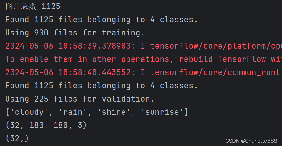
image_count = len(list(data_dir.glob('*/*.jpg')))
print("图片总数",image_count)

roses = list(data_dir.glob('sunrise/*.jpg'))
PIL.Image.open(str(roses[0]))

#将下载数据加载到tf.data.Dataset
batch_size = 32
img_height =180
img_width =180
#训练集
train_ds = tf.keras.preprocessing.image_dataset_from_directory(
    data_dir,
    validation_split=0.2,
    subset="training",
    seed=123,
    image_size=(img_height, img_width),
    batch_size=batch_size
)
#验证集
val_ds = tf.keras.preprocessing.image_dataset_from_directory(
    data_dir,
    validation_split=0.2,
    subset="validation",
    seed=123,
    image_size=(img_height, img_width),
    batch_size=batch_size
)
#输出分类名称
class_names = train_ds.class_names
print(class_names)

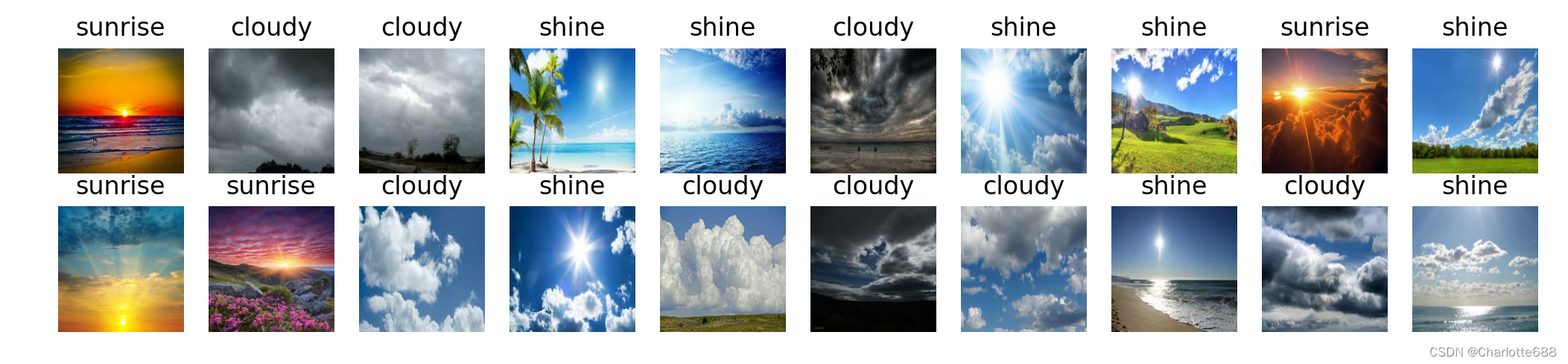
#可视化数据
plt.figure(figsize=(20,10))

for images, labels in train_ds.take(1):
    for i in range(20):
        ax = plt.subplot(5,10,i+1)

        plt.imshow(images[i].numpy().astype("uint8"))
        plt.title(class_names[labels[i]])

        plt.axis("off")

 #输出数据图片张量
for image_batch, labels_batch in train_ds:
    print(image_batch.shape)
    print(labels_batch.shape)
    break

输出

2.建立模型

老演员CNN代码如下：

 #配置数据(打乱数据，预抓取）
AUTOTUNE = tf.data.AUTOTUNE

train_ds =train_ds.cache().shuffle(1000).prefetch(buffer_size=AUTOTUNE)
val_ds = val_ds.cache().prefetch(buffer_size=AUTOTUNE)

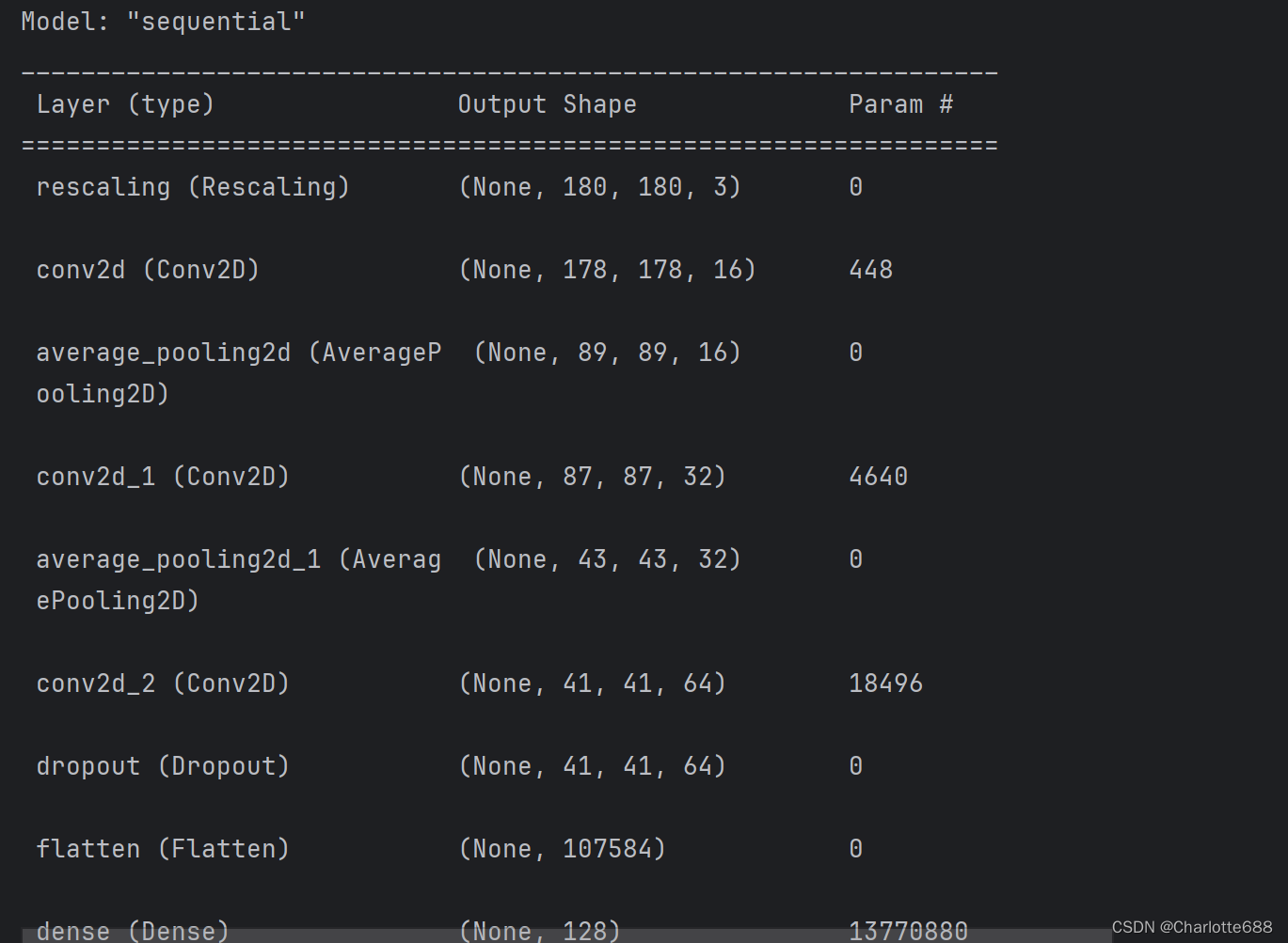
#构建网络CNN老演员
num_classes = 4

model = models.Sequential([
    layers.experimental.preprocessing.Rescaling(1./255, input_shape=(img_height,img_width,3)),

    layers.Conv2D(16,(3,3), activation='relu',input_shape=(img_height, img_width,3)),
    layers.AveragePooling2D((2,2)),
    layers.Conv2D(32,(3,3), activation='relu'),
    layers.AveragePooling2D((2,2)),
    layers.Conv2D(64, (3,3), activation='relu'),
    layers.Dropout(0.3),

    layers.Flatten(),
    layers.Dense(128, activation='relu'),
    layers.Dense(num_classes)
])

model.summary()

输出模型简介

3.编译、训练模型

代码如下：

#设置学习率
opt = tf.keras.optimizers.Adam(learning_rate=0.001)
#编译
model.compile(optimizer=opt,
              loss=tf.keras.losses.SparseCategoricalCrossentropy(from_logits=True),
              metrics=['accuracy'])

epochs = 10

history = model.fit(
    train_ds,
    validation_data=val_ds,
    epochs=epochs
)

3.评估模型并绘制ACC曲线和LOSS曲线

代码如下：

#模型评估
acc = history.history['accuracy']
val_acc = history.history['val_accuracy']

loss = history.history['loss']
val_loss = history.history['val_loss']


epochs_range = range(epochs)
#绘制准确率曲线
plt.figure(figsize=(12,4))
plt.subplot(1,2,1)
plt.plot(epochs_range, acc, label='Training Accuracy')
plt.plot(epochs_range, val_acc, label = 'Validation Accuracy')
plt.legend(loc = 'lower right')
plt.title('Training and Validation Accuracy')
#绘制损失函数曲线
plt.subplot(1, 2, 2)
plt.plot(epochs_range, loss, label = 'Training Loss')
plt.plot(epochs_range, val_loss, label = 'Validation Loss')
plt.legend(loc='upper right')
plt.title('Training and Validation Loss')
plt.show()

输出曲线

---

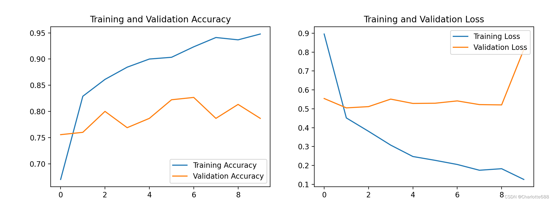
总结

本次主要加入了模型评估环节，并将评估结果可视化