利用matlab mobile采集GPS数据进行可视化分析

Hello啊，GPS数据在交通大数据分析中起到了很大作用，。。。。。（不想写废话了，直接开始吧）

首先，需要在手机上下载matlab移动端，iOS和安卓系统都可以下，我刚开始学习matlab的时候用过，还算好用，需要申请账号什么的就不说了。

下载好之后，直接登录即可。

在传感器页面，就可以看到相应的采集页面，点击开始采集。当关闭后，进入MATHWORK官网个人账户（MATLAB Drive），可下载所采集到的内容。

另一种有效的方式是在命令行创建 mobiledev 对象，将产生一个采集器，开始采集，当采集结束后，关闭即可，原理相同，但采用这种方式，在移动端进行数据处理会方便很多。

m = mobiledev;  % 启动传感器前创建 mobiledev 对象
m.Logging = 1;  % 开始记录数据
m.PositionSensorEnabled = 1;
pause(1000) % 采集时长
m.Logging = 0;  % 停止记录数据

 得到的m为m是采集传感器数据的 mobiledev 对象的名称，matlab提供了各种在移动端处理所得数据的函数。

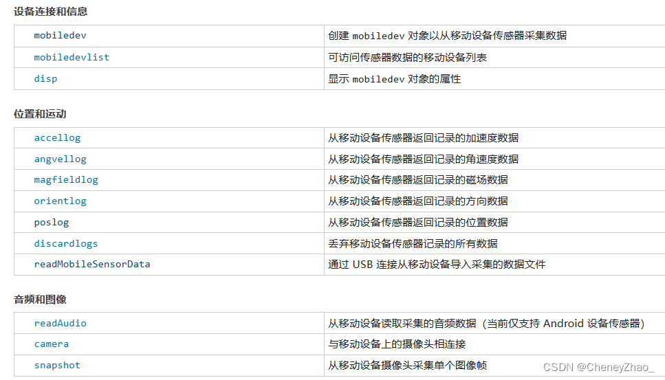
比较常用的函数 用法这里备注下，有需要可去官网自行查看。

[lat, lon, t, speed, course, alt, horizacc] = poslog(m) % 获取记录的纬度、经度、时间戳、速度、航向、海拔和水平精度位置数据

[log, timestamp] = accellog(m) % 返回加速度日志

做了一个可视化工具：

这些数据处理过程将在PC端进行（暂时不知道移动端能不能运行）

首先，我们load一下前面所采集到的数据：

clc;clear
load sensorlog_20230608_171258.mat % 这个是2023年6月8日去学校外卖吃饭采集的数据hhh

由于笔者是做交通运行评价方面的，这里简单以自己研究方向做个可视化分析：

所导入的数据得到的是一个Table数据类型的变量，（之前采集只采集了位置信息，因为暂时只有位置信息对我有用）

我们对数据进行提取：

lat = cell2mat(table2cell(Position(:,'latitude')));
lon = cell2mat(table2cell(Position(:,'longitude')));
speed = cell2mat(table2cell(Position(:,'speed')));

对所得数据进行处理得到轨迹图形(篇幅有限，不对经纬度转距离的函数进行展示了，百度都有)：

[n,~] = size(speed);
set_ao = [lat lon];
begin  = set_ao(1,:);
dist = Dist(begin,set_ao);
time = [1:n]';

sub1 = subplot(1,2,1);
plot(time,dist,'LineWidth',2)
xlabel('Time (s)')
ylabel('Distance (km)');
set(get(gca,'XLabel'),'FontSize',10);
sub2 = subplot(1,2,2);
plot(speed,dist,'-','LineWidth',2)
xlabel('V (m/s)')
set(get(gca,'XLabel'),'FontSize',10);
set(gca,'FontName','Times New Roman','FontSize',10)

pos1 = [0.1,0.097619047619048,0.616071428571429,0.821299871299871];
pos2 = [0.715625,0.097619047619048,0.235785615528263,0.821299871299871];
set(sub2,'Position',pos2)
set(sub1,'Position',pos1)
set(gca,'ytick',[],'yticklabel',[])
sgtitle('Trajectory View on a Time-Space Diagram'); 

得到时空图如图：

下面我们在地图上将行驶轨迹展示出来：

%% 对速度值分 bin 以便使用离散数量的颜色来表示观测到的速度
nBins = 10;
binSpacing = (max(speed) - min(speed))/nBins; 
binRanges = min(speed):binSpacing:max(speed)-binSpacing; 

% Add an inf to binRanges to enclose the values above the last bin.
binRanges(end+1) = inf;

% |histc| determines which bin each speed value falls into.
[~, speedBins] = histc(speed, binRanges);

lat = lat';
lon = lon';
speedBins = speedBins';

% Create a geographical shape vector, which stores the line segments as
% features.
s = geoshape();
%% 为每个速度 bin 创建一个不连续线段。将为每个线段分配一种颜色。
for k = 1:nBins
    
    % Keep only the lat/lon values which match the current bin. Leave the 
    % rest as NaN, which are interpreted as breaks in the line segments.
    latValid = nan(1, length(lat));
    latValid(speedBins==k) = lat(speedBins==k);
    
    lonValid = nan(1, length(lon));
    lonValid(speedBins==k) = lon(speedBins==k);    

    % To make the path continuous despite being segmented into different
    % colors, the lat/lon values that occur after transitioning from the
    % current speed bin to another speed bin will need to be kept.
    transitions = [diff(speedBins) 0];
    insertionInd = find(speedBins==k & transitions~=0) + 1;

    % Preallocate space for and insert the extra lat/lon values.
    latSeg = zeros(1, length(latValid) + length(insertionInd));
    latSeg(insertionInd + (0:length(insertionInd)-1)) = lat(insertionInd);
    latSeg(~latSeg) = latValid;
    
    lonSeg = zeros(1, length(lonValid) + length(insertionInd));
    lonSeg(insertionInd + (0:length(insertionInd)-1)) = lon(insertionInd);
    lonSeg(~lonSeg) = lonValid;

    % Add the lat/lon segments to the geographic shape vector.
    s(k) = geoshape(latSeg, lonSeg);
    
end
%% 使用 webmap 在浏览器中打开一个 Web 地图
wm = webmap('World Imagery');
%% 标记 位置
mwLat = 30.43932;
mwLon = 114.26154;
name = 'MathWorks';
iconDir = fullfile(matlabroot,'toolbox','matlab','icons');
iconFilename = fullfile(iconDir, 'wust.gif');
wmmarker(mwLat, mwLon, 'FeatureName', name, 'Icon', iconFilename);
%% 使用 autumn 颜色图生成与速度 bin 对应的颜色列表。这将为每个 bin 创建一个具有 RGB 值的 [nBins x 3] 矩阵
colors = autumn(nBins);
wmline(s, 'Color', colors, 'Width', 5);
%% 放大地图并聚焦于路线
wmzoom(17);

得到的实际轨迹图如图：

颜色越深表示我走的越慢。 

很简单的小东西，希望对你有帮助。