回归模型的不稳定性

作者：chen_h
微信号 & QQ：862251340
微信公众号：coderpai

---

介绍

由于各种原因，回归系数可能存在且不稳定。这篇文章会简单介绍这种情况。

回归分析允许我们估计函数中的系数，该函数用于设计的多个数据集。我们假设这个函数的一个特定形式，然后找到适合数据的系数，假设偏离模型可以被认为是噪声。

在构建这样的模型时，我们接受它不能完美的预测因变量。在这里，我们想要评估模型的准确性。而不是它如何解释因变量，而是评估我们的样本数据的稳定性（即回归系数的稳定性）。毕竟，如果一个模型真的很合适，那么它应该类似于我们单独建模的两个随机的数据集的模型。否则，我们认为模型仅仅是适合我们选择的特定数据样本的结果。

我们将此处使用线性回归来说明这个问题，但同时也应该适用于所有回归模型。下面我们为 stasmodels 的线性回归定义一个包装函数，以便我们以后可以使用它。

import numpy as np
import pandas as pd
from statsmodels import regression, stats
import statsmodels.api as sm
import matplotlib.pyplot as plt
import scipy as sp

def linreg(X,Y):
    # Running the linear regression
    x = sm.add_constant(X) # Add a row of 1's so that our model has a constant term
    model = regression.linear_model.OLS(Y, x).fit()
    return model.params[0], model.params[1] # Return the coefficients of the linear model

有偏见的噪音

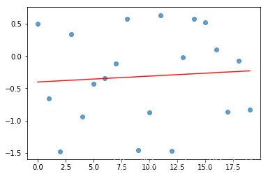
我们为数据选择的特定样本会影响我们生成的模型，不均匀分布的噪声会导致模型不准确。下面我们生成正太分布数据，但由于我们没有很多数据点，因此我们看到了显著的向下偏差。如果我们进行更多测量，那么两个回归系数都将趋向于零。

# Draw observations from normal distribution
np.random.seed(107) # Fix seed for random number generation
rand = np.random.randn(20)

# Conduct linear regression on the ordered list of observations
xs = np.arange(20)
a, b = linreg(xs, rand)
print('Slope:', b, 'Intercept:', a)

# Plot the raw data and the regression line
plt.scatter(xs, rand, alpha=0.7)
Y_hat = xs * b + a
plt.plot(xs, Y_hat, 'r', alpha=0.9);

plt.show()

Slope: 0.009072503822685526 Intercept: -0.40207744085303815

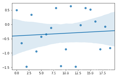
import seaborn

seaborn.regplot(xs, rand)

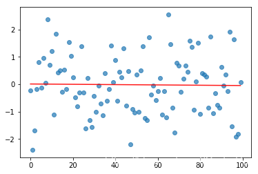
# Draw more observations
rand2 = np.random.randn(100)

# Conduct linear regression on the ordered list of observations
xs2 = np.arange(100)
a2, b2 = linreg(xs2, rand2)
print('Slope:', b2, 'Intercept:', a2)

# Plot the raw data and the regression line
plt.scatter(xs2, rand2, alpha=0.7)
Y_hat2 = xs2 * b2 + a2
plt.plot(xs2, Y_hat2, 'r', alpha=0.9);

plt.show()

Slope: -0.0005693423631053353 Intercept: 0.009011767319021785

回归分析对异常值非常敏感。有时候这些异常值又会包含很多信息，在这种情况下我们要考虑他们。但是，在上述情况下，它们可能只是随机噪音。虽然我们的数据点通常比上面的例子多很多，但我们可能会有（例如）数周或者数月的波动，这会显著改变回归系数。

结构性改变

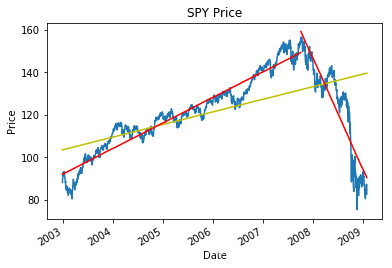
制度变化（或者结构性变化）是指在生成数据的过程中发生变化，导致未来样本遵循不同的分布。下面，我们可以看到在 2007 年底有一个政权更改，并且在那里分割数据导致比整个数据集（黄色）的回归更好（红色）。在这种情况下，我们的回归模型将无法预测未来的数据点，因为底层系统不再与样本中的相同。实际上，回归分析假设误差是不相关的并且具有恒定的方差，如果存在制度变化，则通常不是这种情况。

import pandas_datareader as pdr

start = '2003-01-01'
end = '2009-02-01'
#pricing = get_pricing('SPY', fields='price', start_date=start, end_date=end)
data = pdr.get_data_yahoo('SPY', start = start, end=end)
pricing = data['Close']
# Manually set the point where we think a structural break occurs
breakpoint = 1200
xs = np.arange(len(pricing))
xs2 = np.arange(breakpoint)
xs3 = np.arange(len(pricing) - breakpoint)

# Perform linear regressions on the full data set, the data up to the breakpoint, and the data after
a, b = linreg(xs, pricing)
a2, b2 = linreg(xs2, pricing[:breakpoint])
a3, b3 = linreg(xs3, pricing[breakpoint:])

Y_hat = pd.Series(xs * b + a, index=pricing.index)
Y_hat2 = pd.Series(xs2 * b2 + a2, index=pricing.index[:breakpoint])
Y_hat3 = pd.Series(xs3 * b3 + a3, index=pricing.index[breakpoint:])

# Plot the raw data
pricing.plot()
Y_hat.plot(color='y')
Y_hat2.plot(color='r')
Y_hat3.plot(color='r')
plt.title('SPY Price')
plt.ylabel('Price');

当然，我们打破数据集的碎片越多，我们就越准确的适应它。避免去拟合噪声数据是非常重要的，噪声总是会波动并且不能预测。我们可以在我们已经识别的特定点或一般情况下测试结果中断的存在。下面我们使用来自 statsmodels 的测试，该测试计算在没有断点的情况下观察数据的概率。

stats.diagnostic.breaks_cusumolsresid(
    regression.linear_model.OLS(pricing, sm.add_constant(xs)).fit().resid)[1]

5.713702903582742e-59

多重共线性

上面我们只考虑一个因变量对一个独立变量的回归。但是，我们也可以有多个自变量。如果自变量高度相关，则会导致不稳定。

想象一下，我们使用两个独立变量 $X_1$ 和 $X_2$ ，并且它们具有很高的相关性。然后，如果我们添加一个新的观察结果，那么系数可能会急剧变化，这个观察结果稍微好一点。在极端情况下，如果 $X_1=X_2$ ，则系数的选择将取决于特定的线性回归算法。

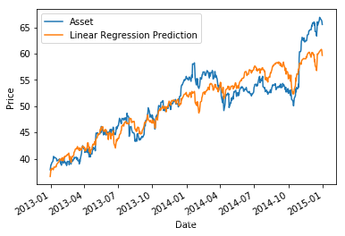
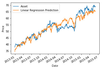
下面，我们运行多元线性回归，其中自变量高度相关。如果我们将采样周期设为 2013-01-01 至 2015-01-01，则系数约为 0.25 和 0.1 ，但如果我们将期限延长至 2015-06-01，则系数分为约为 0.18 和 0.20。

# Get pricing data for two benchmarks (stock indices) and a stock
start = '2013-01-01'
end = '2015-01-01'
#b1 = get_pricing('SPY', fields='price', start_date=start, end_date=end)
#b2 = get_pricing('MDY', fields='price', start_date=start, end_date=end)
#asset = get_pricing('V', fields='price', start_date=start, end_date=end)

data = pdr.get_data_yahoo('SPY', start = start, end=end)
b1 = data['Close']
data = pdr.get_data_yahoo('MDY', start = start, end=end)
b2 = data['Close']
data = pdr.get_data_yahoo('V', start = start, end=end)
asset = data['Close']


mlr = regression.linear_model.OLS(asset, sm.add_constant(np.column_stack((b1, b2)))).fit()
prediction = mlr.params[0] + mlr.params[1]*b1 + mlr.params[2]*b2
print('Constant:', mlr.params[0], 'MLR beta to S&P 500:', mlr.params[1], ' MLR beta to MDY', mlr.params[2])

# Plot the asset pricing data and the regression model prediction, just for fun
asset.plot()
prediction.plot();
plt.ylabel('Price')
plt.legend(['Asset', 'Linear Regression Prediction']);

Constant: -16.243603405890557 MLR beta to S&P 500: 0.2492404646507781  MLR beta to MDY 0.09349176682768158

# Get pricing data for two benchmarks (stock indices) and a stock
start = '2013-01-01'
end = '2015-06-01'

#b1 = get_pricing('SPY', fields='price', start_date=start, end_date=end)
#b2 = get_pricing('MDY', fields='price', start_date=start, end_date=end)
#asset = get_pricing('V', fields='price', start_date=start, end_date=end)

data = pdr.get_data_yahoo('SPY', start = start, end=end)
b1 = data['Close']
data = pdr.get_data_yahoo('MDY', start = start, end=end)
b2 = data['Close']
data = pdr.get_data_yahoo('V', start = start, end=end)
asset = data['Close']

mlr = regression.linear_model.OLS(asset, sm.add_constant(np.column_stack((b1, b2)))).fit()
prediction = mlr.params[0] + mlr.params[1]*b1 + mlr.params[2]*b2
print('Constant:', mlr.params[0], 'MLR beta to S&P 500:', mlr.params[1], ' MLR beta to MDY', mlr.params[2])

# Plot the asset pricing data and the regression model prediction, just for fun
asset.plot()
prediction.plot();
plt.ylabel('Price')
plt.legend(['Asset', 'Linear Regression Prediction']);

Constant: -28.3571287326346 MLR beta to S&P 500: 0.18023806033366943  MLR beta to MDY 0.20011277731901822

我们可以通过计算他们的相关系数来检查我们的自变量是否相关。此数字始终位于 -1 和 1 之间，值 1 表示两个变量完全相关。

# Compute Pearson correlation coefficient
sp.stats.pearsonr(b1,b2)[0] # Second return value is p-value

0.988746070194985

---

来源：quantopian