动手学深度学习Task3

Task3： 线性神经网络

1.线性回归

  线性回归要处理的一类问题是：给定一组输入样本，和每个样本对应的目标值，需要在某一损失准则下，找到（学习到）目标值和输入值的函数关系，这样，当有一个新的样本到达时，可以预测其对应的目标值是多少。
  线性回归包括一元线性回归和多元线性回归
算法步骤：
（1）初始化模型参数的值，如进行随机初始化；
（2）从数据集中随机抽取小批量样本且在负梯度的方向上更新参数，并不断迭代这一步骤。
$$\begin{array}{rl}\mathbf{w}& \leftarrow \mathbf{w}-\frac{\eta }{|\mathcal{B}|}\sum _{i\in \mathcal{B}}{\partial }_{\mathbf{w}}{l}^{(i)}(\mathbf{w},b)=\mathbf{w}-\frac{\eta }{|\mathcal{B}|}\sum _{i\in \mathcal{B}}{\mathbf{x}}^{(i)}\left({\mathbf{w}}^{\top }{\mathbf{x}}^{(i)}+b-y^{(i)}\right),\\ b& \leftarrow b-\frac{\eta }{|\mathcal{B}|}\sum _{i\in \mathcal{B}}{\partial }_b{l}^{(i)}(\mathbf{w},b)=b-\frac{\eta }{|\mathcal{B}|}\sum _{i\in \mathcal{B}}\left({\mathbf{w}}^{\top }{\mathbf{x}}^{(i)}+b-y^{(i)}\right).\end{array}$$
 

2.从零实现线性回归

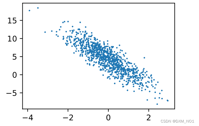
#生成数据集
def synthetic_data(w, b, num_examples):  #@save
    """生成y=Xw+b+噪声"""
    X = torch.normal(0, 1, (num_examples, len(w)))
    y = torch.matmul(X, w) + b
    y += torch.normal(0, 0.01, y.shape)
    return X, y.reshape((-1, 1))
  
true_w = torch.tensor([2, -3.4])
true_b = 4.2
features, labels = synthetic_data(true_w, true_b, 1000)
d2l.set_figsize()
d2l.plt.scatter(features[:, 1].detach().numpy(), labels.detach().numpy(), 1);

# 初始化参数
w = torch.normal(0, 0.01, size=(2,1), requires_grad=True)
b = torch.zeros(1, requires_grad=True)

# 定义模型
def linreg(X, w, b):  #@save
    """线性回归模型"""
    return torch.matmul(X, w) + b
  
# 损失函数
def squared_loss(y_hat, y):  #@save
    """均方损失"""
    return (y_hat - y.reshape(y_hat.shape)) ** 2 / 2
# 优化算法
def sgd(params, lr, batch_size):  #@save
    """小批量随机梯度下降"""
    with torch.no_grad():
        for param in params:
            param -= lr * param.grad / batch_size
            param.grad.zero_()
# 训练
lr = 0.03
num_epochs = 3
net = linreg
loss = squared_loss
batch_size = 10

for epoch in range(num_epochs):
    for X, y in data_iter(batch_size, features, labels):
        l = loss(net(X, w, b), y)  # X和y的小批量损失
        # 因为l形状是(batch_size,1)，而不是一个标量。l中的所有元素被加到一起,
        # 并以此计算关于[w,b]的梯度
        l.sum().backward()
        sgd([w, b], lr, batch_size)  # 使用参数的梯度更新参数
    with torch.no_grad():
        train_l = loss(net(features, w, b), labels)
        print(f'epoch {epoch + 1}, loss {float(train_l.mean()):f}')

 

3.softmax

  softmax函数能够将未规范化的预测变换为非负数并且总和为1，同时让模型保持可导的性质。为了完成这一目标，我们首先对每个未规范化的预测求幂，这样可以确保输出非负。softmax函数定义：
$$\hat{\mathbf{y}}=\mathrm{softmax}(\mathbf{o})\text{其中}{\hat{y}}_j=\frac{\exp (o_j)}{{\sum }_k\exp (o_k)}$$
  通过Softmax函数就可以将多分类的输出值转换为范围在[0, 1]和为1的概率分布。
  softmax函数定义：

def softmax(X):
    X_exp = torch.exp(X)
    partition = X_exp.sum(1, keepdim=True)
    return X_exp / partition  # 这里应用了广播机制

  

softmax回归的从零开始实现

引入MNIST数据集

import torch
from IPython import display
from d2l import torch as d2l

batch_size = 256
train_iter, test_iter = d2l.load_data_fashion_mnist(batch_size)

初始化模型参数

num_inputs = 784
num_outputs = 10

W = torch.normal(0, 0.01, size=(num_inputs, num_outputs), requires_grad=True)
b = torch.zeros(num_outputs, requires_grad=True)

X = torch.tensor([[1.0, 2.0, 3.0], [4.0, 5.0, 6.0]])
X.sum(0, keepdim=True), X.sum(1, keepdim=True)

定义softmax

def softmax(X):
    X_exp = torch.exp(X)
    partition = X_exp.sum(1, keepdim=True)
    return X_exp / partition  # 这里应用了广播机制

定义模型

def net(X):
    return softmax(torch.matmul(X.reshape((-1, W.shape[0])), W) + b)
Copy to clipboard

定义损失函数

def cross_entropy(y_hat, y): #这里是交叉熵损失函数
    return - torch.log(y_hat[range(len(y_hat)), y])

分类精度

def accuracy(y_hat, y):  #@save
    """计算预测正确的数量"""
    if len(y_hat.shape) > 1 and y_hat.shape[1] > 1:
        y_hat = y_hat.argmax(axis=1)
    cmp = y_hat.type(y.dtype) == y
    return float(cmp.type(y.dtype).sum())

训练

def train_epoch_ch3(net, train_iter, loss, updater):  #@save
    """训练模型一个迭代周期（定义见第3章）"""
    # 将模型设置为训练模式
    if isinstance(net, torch.nn.Module):
        net.train()
    # 训练损失总和、训练准确度总和、样本数
    metric = Accumulator(3)
    for X, y in train_iter:
        # 计算梯度并更新参数
        y_hat = net(X)
        l = loss(y_hat, y)
        if isinstance(updater, torch.optim.Optimizer):
            # 使用PyTorch内置的优化器和损失函数
            updater.zero_grad()
            l.mean().backward()
            updater.step()
        else:
            # 使用定制的优化器和损失函数
            l.sum().backward()
            updater(X.shape[0])
        metric.add(float(l.sum()), accuracy(y_hat, y), y.numel())
    # 返回训练损失和训练精度
    return metric[0] / metric[2], metric[1] / metric[2]

预测

def predict_ch3(net, test_iter, n=6):  #@save
    """预测标签（定义见第3章）"""
    for X, y in test_iter:
        break
    trues = d2l.get_fashion_mnist_labels(y)
    preds = d2l.get_fashion_mnist_labels(net(X).argmax(axis=1))
    titles = [true +'\n' + pred for true, pred in zip(trues, preds)]
    d2l.show_images(
        X[0:n].reshape((n, 28, 28)), 1, n, titles=titles[0:n])

predict_ch3(net, test_iter)