逻辑回归实践

逻辑回归实践

数据准备

(1)生成200条二分类数据（2个特征）

from sklearn.datasets import make_blobs
X, y = make_blobs(n_samples = 200, 
                      n_features = 2,
                      centers = 2,
                      random_state = 8)

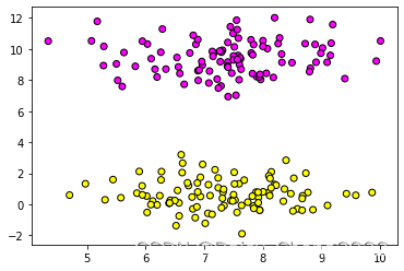
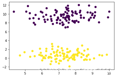
(2)数据可视化

import matplotlib.pyplot as plt
%matplotlib inline
plt.scatter(X[:, 0], X[:, 1], c = y, cmap = plt.cm.spring, edgecolors = 'k')

plt.scatter(X[:, 0], X[:, 1], c = y)

梯度下降法实现逻辑回归（批量，平均，随机）

(1)数据准备

import numpy as np

# 添加全1列
x_ones = np.ones((X.shape[0], 1))             
X = np.hstack((X, x_ones))

#拆分数据
from sklearn.model_selection import train_test_split
X_train, X_test, y_train, y_test = train_test_split(X, y, test_size = 0.3, random_state = 8)

(2)查看数据维度

print(X.shape, X_train.shape, X_test.shape)
print(y.shape, y_train.shape, y_test.shape)

(3)将因变量转为列向量

y_train = y_train.reshape(-1, 1)
y_test = y_test.reshape(-1, 1)
print(y_train.shape, y_test.shape)

(4)定义sigmoid函数

#初始化theta值
theta = np.ones([X_train.shape[1], 1])
alpha = 0.001

#定义sigmoid函数        
def sigmoid(z):
    s = 1.0 / (1 + np.exp(-z))
    return s

(5)预测

num_iters = 10000
m = 140   #对应训练集数据数
for i in range(num_iters):
    h = sigmoid(np.dot(X_train, theta))
    theta = theta - alpha * np.dot(X_train.T, (h - y_train)) / m
print(theta)

#预测
pred_y = sigmoid(np.dot(X_test, theta))

#预测结果二值化
pred_y[pred_y > 0.5] = 1
pred_y[pred_y <= 0.5] = 0
print(pred_y.reshape(1, -1))
print(y_test.reshape(1, -1))

print('预测准确率为：', np.sum(pred_y == y_test) / len(y_test))

kaggle糖尿病预测实战

(1)数据准备

#导入数据
import pandas as pd
data = pd.read_csv('pima-indians-diabetes.data.csv')
print(data)

#分离特征变量和分类变量
X = data.iloc[:, :-1]
y = data.iloc[:, -1]

#特征标准化
mu = X.mean(axis = 0)
std = X.std(axis = 0)
X = (X - mu) / std

#添加全1列
x_ones = np.ones((X.shape[0], 1))
X = np.hstack((X, x_ones))

#拆分训练集和测试集
X_train, X_test, y_train, y_test = train_test_split(X, y, test_size = 0.3, random_state = 8)

#将因变量转为列向量
y_train = y_train.values.reshape(-1, 1)
y_test = y_test.values.reshape(-1, 1)

print(y_train.shape, y_test.shape)

(2)定义sigmoid函数

#初始化theta值
theta = np.ones([X_train.shape[1], 1])
alpha = 0.001

#定义sigmoid函数         #问题：logistic函数是什么
def sigmoid(z):
    s = 1.0 / (1 + np.exp(-z))
    return s

(3)预测

num_iters = 10000
m = 537  #对应训练集个数
for i in range(num_iters):
    h = sigmoid(np.dot(X_train, theta))
    theta = theta - alpha * np.dot(X_train.T, (h - y_train)) / m
print(theta)

#预测
pred_y = sigmoid(np.dot(X_test, theta))

#预测结果二值化
pred_y[pred_y > 0.5] = 1
pred_y[pred_y <= 0.5] = 0
print(pred_y.reshape(1, -1))
print(y_test.reshape(1, -1))

print('预测准确率为：', np.sum(pred_y == y_test) / len(y_test))

sklearn实现逻辑回归

逻辑回归实现三分类

(1)数据准备

#导入iris数据集
from sklearn.datasets import load_iris
iris = load_iris()

#分离自变量、因变量
X = iris.data
y = iris.target

#拆分训练集与测试集
from sklearn.model_selection import train_test_split
X_train, X_test, y_train, y_test = train_test_split(X, y, random_state = 8)

(2)导入逻辑回归模块训练

from sklearn.linear_model import LogisticRegression

#三板斧
logis = LogisticRegression()
logis.fit(X_train, y_train)

#查看模型参数设置
logis.get_params()

(3)模型评估

print(logis.score(X_test, y_test))

from sklearn.metrics import classification_report
print(classification_report(y_test, logis.predict(X_test)))

(4)更换参数查看模型效果

#等价于选择参数：multi_class = 'multinomial', solver = 'lbfgs'
logis2 = LogisticRegression(multi_class='multinomial', solver='lbfgs')
logis2.fit(X_train, y_train)

print(logis2.score(X_test, y_test))

#若选择参数：multi_class = 'ovr', solver = 'lbfgs'
logis3 = LogisticRegression(multi_class='ovr', solver='lbfgs')
logis3.fit(X_train, y_train)

logis3.score(X_test, y_test)