


本文没有使用现有的框架,仅使用最原始的代码创建神经网络实现对sin函数的学习。
1.导入相关库
import numpy as np
import matplotlib.pyplot as plt
2.准备输入数据和正确答案数据(对应的label)
input_data = np.arange(0, np.pi*2, 0.1)    #输入
correct_data = np.sin(input_data)          #对应的label
input_data = (input_data-np.pi)/np.pi       #将输入收敛到-1.0~1.0的范围之内
n_data = len(correct_data)                 #数据数量
3.各个设定值
n_in = 1                #输入层的神经元数量
n_mid = 3               #中间层的神经元数量
n_out = 1               #输出层的神经元数量

wb_width = 0.01         #权重和偏置的扩散程度
eta = 0.1               #学习系数
epoch = 2001            #迭代次数
interval = 200          #显示进度的间隔实践
4.中间层
class MiddleLayer:
    def __init__(self, n_upper, n):                        #初始化设置
        self.w = wb_width * np.random.randn(n_upper, n)    #权重(矩阵)
        self.b = wb_width * np.random.randn(n)             #偏置(向量)

    def forward(self, x):                                  #正向传播
        self.x = x
        u = np.dot(x, self.w) + self.b
        self.y = 1/(1 + np.exp(-u))                        #sigmoid函数

    def backward(self, grad_y):
        delta = grad_y * (1 - self.y) * self.y             #sigmoid函数的微分

        self.grad_w = np.dot(self.x.T, delta)
        self.grad_b = np.sum(delta, axis = 0)

        self.grad_x = np.dot(delta, self.w.T)

    def update(self, delta):                               #权重和偏置的更新
        self.w -= eta * self.grad_w
        self.b -= eta * self.grad_b
5.输出层
class OutputLayer:
    def __init__(self, n_upper, n):                        #初始化设置
        self.w = wb_width * np.random.randn(n_upper, n)    #权重(矩阵)
        self.b = wb_width * np.random.randn(n)             #偏置(向量)

    def forward(self, x):                                  #正向传播
        self.x = x
        u = np.dot(x, self.w) + self.b
        self.y = u                                         #恒等函数

    def backward(self, t):                                 #反向传播
        delta = self.y - t

        self.grad_w = np.dot(self.x.T, delta)
        self.grad_b = np.sum(delta, axis = 0)

        self.grad_x = np.dot(delta, self.w.T)

    def update(self, delta):                               #权重和偏置的更新
        self.w -= eta * self.grad_w
        self.b -= eta * self.grad_b
6.各个网络层的初始化
middle_layer = MiddleLayer(n_in, n_mid)
output_layer = OutputLayer(n_mid, n_out)
7.神经网络学习
for i in range(epoch):

    #随机打乱索引值
    index_random = np.arange(n_data)
    np.random.shuffle(index_random)

    #用于结果的显示
    total_error = 0
    plot_x = []
    plot_y = []

    for idx in index_random:
        x = input_data[idx:idx+1]
        t = correct_data[idx:idx+1]

        #正向传播
        middle_layer.forward(x.reshape(1,1))        #将输入转换为矩阵
        output_layer.forward(middle_layer.y)

        #反向传播
        output_layer.backward(t.reshape(1,1))       #将正确答案转为矩阵
        middle_layer.backward(output_layer.grad_x)

        #权重和偏置的更新
        middle_layer.update(eta)
        output_layer.update(eta)

        if i%interval == 0:

            y = output_layer.y.reshape(-1)

            #误差的计算
            total_error += 1.0/2.0 * np.sum(np.square(y-t))    #平方和误差

            plot_x.append(x)
            plot_y.append(y)

    if i%interval == 0:

        plt.plot(input_data, correct_data, linestyle = "dashed")
        plt.scatter(plot_x, plot_y, marker = "+")
        plt.show()

        print("Epoch:" + str(i) + "/" + str(epoch),
                "Error:" + str(total_error/n_data))
完整代码:
import numpy as np
import matplotlib.pyplot as plt

input_data = np.arange(0, np.pi*2, 0.1)    #输入
correct_data = np.sin(input_data)          #对应的label
input_data = (input_data-np.pi)/np.pi       #将输入收敛到-1.0~1.0的范围之内
n_data = len(correct_data)                 #数据数量

n_in = 1                #输入层的神经元数量
n_mid = 3               #中间层的神经元数量
n_out = 1               #输出层的神经元数量

wb_width = 0.01         #权重和偏置的扩散程度
eta = 0.1               #学习系数
epoch = 2001            #迭代次数
interval = 200          #显示进度的间隔实践


class MiddleLayer:
    def __init__(self, n_upper, n):  # 初始化设置
        self.w = wb_width * np.random.randn(n_upper, n)  # 权重(矩阵)
        self.b = wb_width * np.random.randn(n)  # 偏置(向量)

    def forward(self, x):  # 正向传播
        self.x = x
        u = np.dot(x, self.w) + self.b
        self.y = 1 / (1 + np.exp(-u))  # sigmoid函数

    def backward(self, grad_y):
        delta = grad_y * (1 - self.y) * self.y  # sigmoid函数的微分

        self.grad_w = np.dot(self.x.T, delta)
        self.grad_b = np.sum(delta, axis=0)

        self.grad_x = np.dot(delta, self.w.T)

    def update(self, delta):  # 权重和偏置的更新
        self.w -= eta * self.grad_w
        self.b -= eta * self.grad_b


class OutputLayer:
    def __init__(self, n_upper, n):  # 初始化设置
        self.w = wb_width * np.random.randn(n_upper, n)  # 权重(矩阵)
        self.b = wb_width * np.random.randn(n)  # 偏置(向量)

    def forward(self, x):  # 正向传播
        self.x = x
        u = np.dot(x, self.w) + self.b
        self.y = u  # 恒等函数

    def backward(self, t):  # 反向传播
        delta = self.y - t

        self.grad_w = np.dot(self.x.T, delta)
        self.grad_b = np.sum(delta, axis=0)

        self.grad_x = np.dot(delta, self.w.T)

    def update(self, delta):  # 权重和偏置的更新
        self.w -= eta * self.grad_w
        self.b -= eta * self.grad_b


middle_layer = MiddleLayer(n_in, n_mid)
output_layer = OutputLayer(n_mid, n_out)

for i in range(epoch):

    # 随机打乱索引值
    index_random = np.arange(n_data)
    np.random.shuffle(index_random)

    # 用于结果的显示
    total_error = 0
    plot_x = []
    plot_y = []

    for idx in index_random:
        x = input_data[idx:idx + 1]
        t = correct_data[idx:idx + 1]

        # 正向传播
        middle_layer.forward(x.reshape(1, 1))  # 将输入转换为矩阵
        output_layer.forward(middle_layer.y)

        # 反向传播
        output_layer.backward(t.reshape(1, 1))  # 将正确答案转为矩阵
        middle_layer.backward(output_layer.grad_x)

        # 权重和偏置的更新
        middle_layer.update(eta)
        output_layer.update(eta)

        if i%interval == 0:
            y = output_layer.y.reshape(-1)

            # 误差的计算
            total_error += 1.0 / 2.0 * np.sum(np.square(y - t))  # 平方和误差

            plot_x.append(x)
            plot_y.append(y)

    if i%interval == 0:
        plt.plot(input_data, correct_data, linestyle="dashed")
        plt.scatter(plot_x, plot_y, marker="+")
        plt.show()

        print("Epoch:" + str(i) + "/" + str(epoch),
              "Error:" + str(total_error / n_data))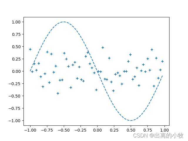


 345
345


 被折叠的 条评论
为什么被折叠?
被折叠的 条评论
为什么被折叠?
 到【灌水乐园】发言


