主成分分析 - 示例代码

主成分分析 - 示例代码

简单介绍

主成分分析就是通过对研究对象的所有维特征进行分析，并找出能够表现出数据特征的最主要的特征，并对特征进行降维度。

其原理是对特征的协方差矩阵进行研究。协方差矩阵可以类比一维的协方差来理解，方差的值对应矩阵中的这一维的特征值。因此找出最大的协方差，就说明这两个维度的差别越大，也就说明其携带的信息就更多。

具体的解释可以如下图所示：

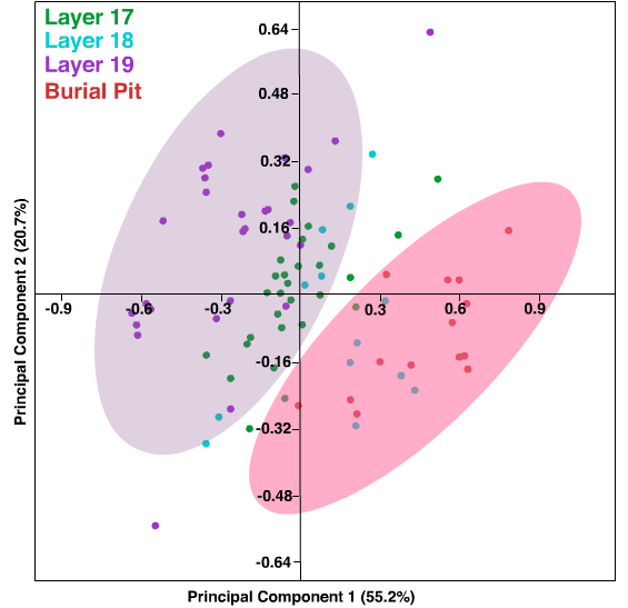
以上数据点有两个主要的特征，紫色和粉色，这两个特征明显可以表现出样本的大部分分布趋势，那么我们就通过对这两个方向进行投影的方式来将空间投影到最有用的两个特征上来进行分析。这样可以大幅度地降低特征的维度！

示例代码

# 方法一： 直接使用现成函数
np.random.seed(1)
n = 1  # The amount of the correlation
x = np.random.uniform(1,2,1000) # Generate 1000 samples from a uniform random variable
y = x.copy() * n # Make y = n * x

# PCA works better if the data is centered

x = x - np.mean(x) # Center x. Remove its mean
y = y - np.mean(y) # Center y. Remove its mean

data = pd.DataFrame({'x': x, 'y': y}) # Create a data frame with x and y
plt.scatter(data.x, data.y) # Plot the original correlated data in blue

pca = PCA(n_components=2) # Instantiate a PCA. Choose to get 2 output variables

# Create the transformation model for this data. Internally, it gets the rotation 

# matrix and the explained variance

pcaTr = pca.fit(data)

rotatedData = pcaTr.transform(data) # Transform the data base on the rotation matrix of pcaTr

# # Create a data frame with the new variables. We call these new variables PC1 and PC2

dataPCA = pd.DataFrame(data = rotatedData, columns = ['PC1', 'PC2']) 

# Plot the transformed data in orange

plt.scatter(dataPCA.PC1, dataPCA.PC2)
plt.show()


#  方法二 使用使用PCA的基本算法

# UNQ_C5 GRADED FUNCTION: compute_pca

def compute_pca(X, n_components=2):
    """
    Input:
        X: of dimension (m,n) where each row corresponds to a word vector
        n_components: Number of components you want to keep.
    Output:
        X_reduced: data transformed in 2 dims/columns + regenerated original data
    pass in: data as 2D NumPy array
    """

### START CODE HERE ###
# mean center the data
X_demeaned = X- np.mean(X,axis=0)

# calculate the covariance matrix
covariance_matrix = np.cov(X_demeaned.T)

# calculate eigenvectors & eigenvalues of the covariance matrix
eigen_vals, eigen_vecs = np.linalg.eigh(covariance_matrix)

# sort eigenvalue in increasing order (get the indices from the sort)
idx_sorted = np.argsort(eigen_vals)

# reverse the order so that it's from highest to lowest.
idx_sorted_decreasing = idx_sorted[::-1]

# sort the eigen values by idx_sorted_decreasing
eigen_vals_sorted = eigen_vals[idx_sorted_decreasing]

# sort eigenvectors using the idx_sorted_decreasing indices
eigen_vecs_sorted = eigen_vecs[:,idx_sorted_decreasing]

# select the first n eigenvectors (n is desired dimension
# of rescaled data array, or dims_rescaled_data)
eigen_vecs_subset = eigen_vecs_sorted[:,0:n_components]

# transform the data by multiplying the transpose of the eigenvectors with the transpose of the de-meaned data
# Then take the transpose of that product.
X_reduced = np.dot(eigen_vecs_subset.T,X_demeaned.T).T

### END CODE HERE ###

return X_reduced