20232402 2023-2024-2 《Python程序设计》实验四报告

20232402王艺瑶

已于 2024-05-30 16:22:09 修改

阅读量969

点赞数 35

文章标签： python

于 2024-05-30 16:20:57 首次发布

本文链接：https://blog.csdn.net/Diligence____/article/details/139273978

版权

20232402 2023-2024-2 《Python程序设计》实验四报告

课程：《Python程序设计》
班级： 2324
姓名：王艺瑶
学号：20232402
实验教师：王志强
实验日期：2024年5月15日
必修/选修：公选课

1.实验内容

训练一个能够通过图片识别衣服类型的模型
数据集：Fashion MNIST
模型：简单的卷积神经网络（CNN）
环境：CPU上运行，使用TensorFlow-Keras

2. 实验过程——model.py

2.1 引用软件包

tensorflow.keras 是 TensorFlow 中的一个高级API，它是由Google开发的开源机器学习框架，用于构建和训练深度学习模型。
matplotlib.pyplot是Python中用于绘制图表和可视化数据的库的一部分。它提供了类似于MATLAB的绘图接口，能够创建各种类型的图表，包括折线图、散点图、直方图等
NumPy是Python中用于科学计算的一个库，它提供了一个强大的多维数组对象和用于处理这些数组的函数，可以执行各种数学运算，例如数组操作、线性代数、傅立叶变换和随机数生成等。

import numpy as np
from tensorflow.keras import datasets, layers, models
import matplotlib.pyplot as plt

2.2 引用并预处理数据集

数据集介绍：
Fashion-MNIST是一个用于机器学习和计算机视觉研究的经典数据集。数据集中包含已经预先划分好的训练集和测试集，其中训练集共60,000张图像，测试集共10,000张图像。每张图像均为单通道黑白图像，大小为28*28pixel，分属10个类别：T-Shirt/Top（T恤），Trouser（裤子），Pullover（套衫），Dress（连衣裙），Coat（大衣），Sandals（凉鞋），Shirt（衬衣），Sneaker（运动鞋），Bag（包），Ankle boots（踝靴）。

2.2.1 加载Fashion MNIST数据集

(train_images, train_labels), (test_images, test_labels) = datasets.fashion_mnist.load_data()

2.2.2 列出类别名称

name = ['T 恤/上衣', '裤子', '套头衫', '连衣裙', '外套', '凉鞋', '衬衫', '运动鞋', '包', '短靴']

2.2.3 图像归一化

通过将每个像素值除以255，可以将其归一化到0到1的范围内，这有助于模型更有效地进行训练和预测。

train_images = train_images / 255.0
test_images = test_images / 255.0

2.2.4 为CNN添加颜色通道

添加颜色通道是为了与卷积神经网络（CNN）的输入格式相匹配。CNN通常接受形状为(图像数量, 宽度, 高度, 通道数)的输入数据。

train_images = train_images.reshape((train_images.shape[0], 28, 28, 1))
test_images = test_images.reshape((test_images.shape[0], 28, 28, 1))

2.3 构建卷积神经网络

2.3.1 构建序列模型

序列模型是一种简单的神经网络模型，它由一系列层按顺序连接而成，数据流从输入经过每一层逐步转换，最终得到输出。适用于图像分类。

model = (models.Sequential
([
    layers.Conv2D(32, (3, 3), activation='relu', input_shape=(28, 28, 1)),  # 第一层卷积层，Relu激活函数
    layers.MaxPooling2D((2, 2)),  # 最大池化层，降低图的空间尺寸
    layers.Conv2D(64, (3, 3), activation='relu'),  # 第二层卷积层
    layers.MaxPooling2D((2, 2)),
    layers.Flatten(),  # 将多维数据展平为一维，为全连接层做准备
    layers.Dense(64, activation='relu'),  # 全连接层
    layers.Dense(10, activation='softmax')  # 输出层，softmax激活函数输出分类概率分布
]))

2.3.2 编译模型

编译模型是为了配置模型的学习过程。包括指定优化器（决定模型如何更新参数以最小化损失函数）、损失函数（用于衡量模型在训练过程中的性能）和评估指标（训练过程中监控模型的性能。）。

model.compile(optimizer='adam',  # 优化器
              loss='sparse_categorical_crossentropy',  # 损失函数为稀疏分类交叉熵
              metrics=['accuracy'])  # 评估指标为准确率

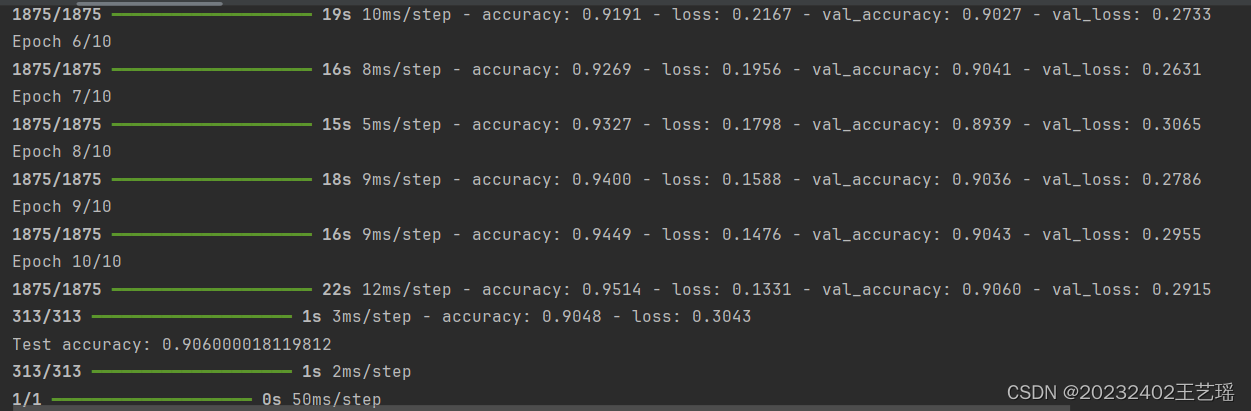
2.4 训练模型

model.fit 函数会将输入数据（train_images 和 train_labels）提供给模型，并进行多次迭代的训练。每次迭代中，模型会根据给定的数据和损失函数调整自己的参数，以最小化损失函数。训练完成后，该函数返回一个 history 对象，其中包含了训练过程中的损失值和其他指定的评估指标值的历史记录。

history = model.fit(train_images, train_labels,
                    epochs=10,  # 十轮
                    validation_data=(test_images, test_labels))

2.5 评估模型

test_loss, test_acc = model.evaluate(test_images, test_labels)
print(f"Test accuracy: {test_acc}")  # f-string 格式化输出

2.6 可视化训练过程

# 绘制训练和验证的准确率曲线
plt.plot(history.history['accuracy'], label='accuracy')  # 训练集准确率曲线
plt.plot(history.history['val_accuracy'], label = 'val_accuracy')  # 测试集
plt.xlabel('Epoch')  # x轴标签
plt.ylabel('Accuracy')
plt.ylim([0, 1])  # y轴的取值范围为0到1
plt.legend(loc='lower right')  # 设置图例显示在右下角
plt.show()

2.7 预测并绘制图像

# 预测
pre = model.predict(test_images)

# 显示图像及其预测结果
def plot_image(i, prearray, trlabel, img):  # 获取第i个样本的预测数组、真实标签和图像
    prearray, trlable, img = prearray[i], trlabel[i], img[i]
    plt.grid(False)  # 关闭网格
    plt.xticks([])   # 移除x轴刻度
    plt.yticks([])
    plt.imshow(img[...,0], cmap=plt.cm.binary)  # 显示图像，使用二值化颜色映射
    prelabel = np.argmax(prearray)
    if prelabel == trlabel:
        color = 'blue'
    else:
        color = 'red'

    plt.xlabel("{} {:2.0f}% ({})".format(name[prelabel],
                                         100*np.max(prearray),
                                         name[trlabel]),
                                         color=color)   #f_string

# 显示各个类别的预测概率
def plot_value_array(i, prearray, trlabel):
    prearray, trlabel = prearray[i], trlabel[i]
    plt.grid(False)
    plt.xticks(range(10))  # 设置x轴刻度为0-9
    plt.yticks([])
    thisplot = plt.bar(range(10), prearray, color="#777777")  # 绘制条形图，显示每个类别的预测概率，颜色设置为灰色
    plt.ylim([0, 1])
    prelabel = np.argmax(prearray)

    thisplot[prelabel].set_color('red')  # 将预测标签对应的条形图颜色设为红色
    thisplot[trlabel].set_color('blue')  # 将真实标签对应的条形图颜色设为蓝色
    
# 显示各个类别的预测概率
def plot_value_array(i, prearray, trlabel):
    prearray, trlabel = prearray[i], trlabel[i]
    plt.grid(False)
    plt.xticks(range(10))  # 设置x轴刻度为0-9
    plt.yticks([])
    thisplot = plt.bar(range(10), prearray, color="#777777")  # 绘制条形图，显示每个类别的预测概率，颜色设置为灰色
    plt.ylim([0, 1])
    prelabel = np.argmax(prearray)

    thisplot[prelabel].set_color('red')  # 将预测标签对应的条形图颜色设为红色
    thisplot[trlabel].set_color('blue')  # 将真实标签对应的条形图颜色设为蓝色

2.8 保存模型

model.save('model.keras')

3.实验过程——classify.py

3.1 引入库并加载模型

import tkinter as tk
from tkinter import filedialog, Label
from tkinterdnd2 import DND_FILES, TkinterDnD
from PIL import Image, ImageTk
import numpy as np
from tensorflow.keras.models import load_model
from model import name

# 加载模型
model = load_model('model.keras')

3.2 图像预处理

def preprocessing(image_path):
    img = Image.open(image_path).convert('L')  # 转换为灰度图像（'L'表示灰度）
    img = img.resize((28, 28))  # 大小调整为28x28像素
    img = np.array(img) / 255.0  # 将图像转换为NumPy数组，并进行归一化处理
    img = img.reshape(1, 28, 28, 1)  # 其中1表示样本数，28x28表示图像大小，1表示通道数（灰度图像只有一个通道）
    return img

3.3 调整图像大小并保持纵横比

def resize_image(image, new_width, new_height):
    aspect_ratio = image.width / image.height
    if aspect_ratio > 1:  # 宽图像
        new_height = int(new_width / aspect_ratio)
    else:  # 窄图像
        new_width = int(new_height * aspect_ratio)

    resized_image = image.resize((new_width, new_height), Image.LANCZOS)  # Image.LANCZOS 过滤器进行高质量缩放
    return resized_image

3.4 分类

# 分类
def classify(image_path):
    img = preprocessing(image_path)
    prediction = model.predict(img)  # 使用模型进行预测
    pre_class = name[np.argmax(prediction)]  # 获取预测的类别

    img_dis = Image.open(image_path)
    img_dis = resize_image(img_dis, 400, 300)  # 调整图像大小为400x300像素
    tk_img = ImageTk.PhotoImage(img_dis)  # 转换成Tkinter格式
    panel.config(image=tk_img)  # 更新Label组件显示的图像
    panel.image = tk_img  # 绑定新的图像对象到Label组件上

    result.config(text=f"Prediction: {pre_class}")  # 更新结果标签

3.5 文件选择或拖放上传

def upload_file():
    file_path = filedialog.askopenfilename()
    if file_path:
        classify(file_path)
def drop(event):
    file_path = event.data
    classify(file_path)

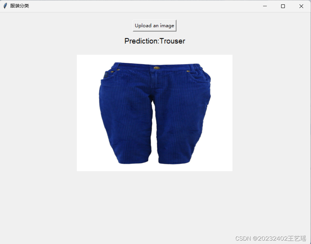
3.6 创建交互界面

# 创建主窗口
root = TkinterDnD.Tk()
root.title("服装分类")
root.geometry("800x600")

# 创建Canvas背景和组件
canvas = tk.Canvas(root, width=800, height=600)  # 创建Canvas来放置背景
canvas.pack(fill='both', expand=True)

bg_path = "background.png"
bg = Image.open(bg_path)
bg = resize_image(bg, 800, 600)  # 调整背景图像大小为窗口大小
bg_photo = ImageTk.PhotoImage(bg)
canvas.create_image(0, 0, image=bg_photo, anchor='nw')

frame = tk.Frame(root, bg='white', bd=5)
canvas.create_window(400, 50, window=frame, anchor="n")  # window 参数指定要嵌入到 Canvas 中的窗口小部件

# 添加按钮和标签
button = tk.Button(frame, text="Upload an image", command=upload_file, font=('Helvetica', 12))  # 按钮
button.grid(row=0, column=0)

result = Label(frame, text="Prediction: ", font=('Helvetica', 14), bg='white')  # 结果标签
result.grid(row=0, column=1)

panel = Label(canvas, bg='white')  # 在Canvas上放置用于显示图像的Label
canvas.create_window(400, 300, window=panel)  # 位置根据需要调整

# 绑定拖放事件
root.drop_target_register(DND_FILES)  # 绑定拖拽事件
root.dnd_bind('<<Drop>>', drop)

4.实验结果

4.1 测试结果

![测试图像](https://img-blog.csdnimg.cn/direct/2482fcc0eaf94589999c22ada99b96d7.pn

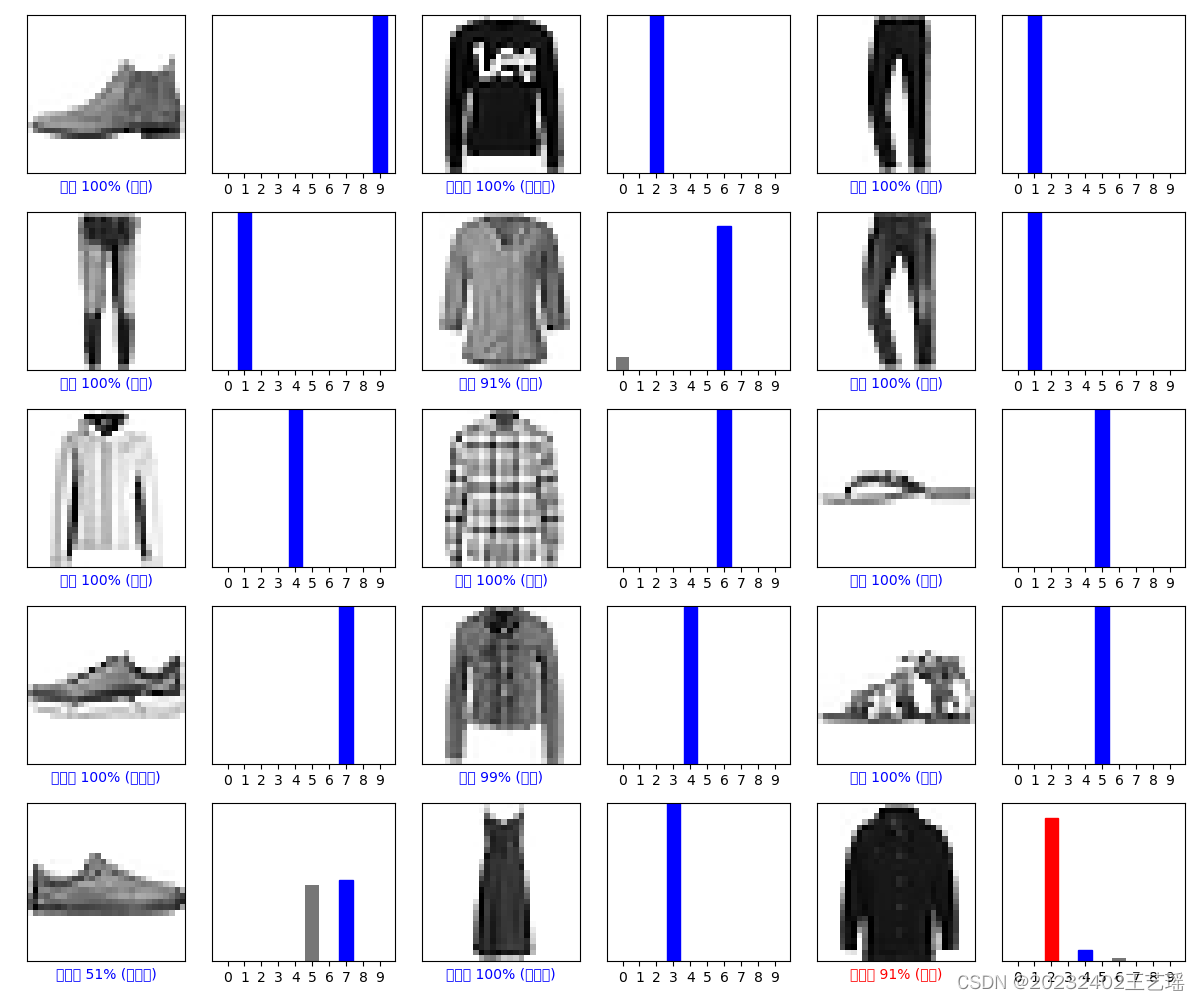
随着epoch增加的训练和测试的准确性曲线

在这里插入图片描述

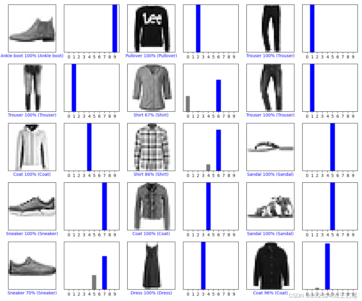
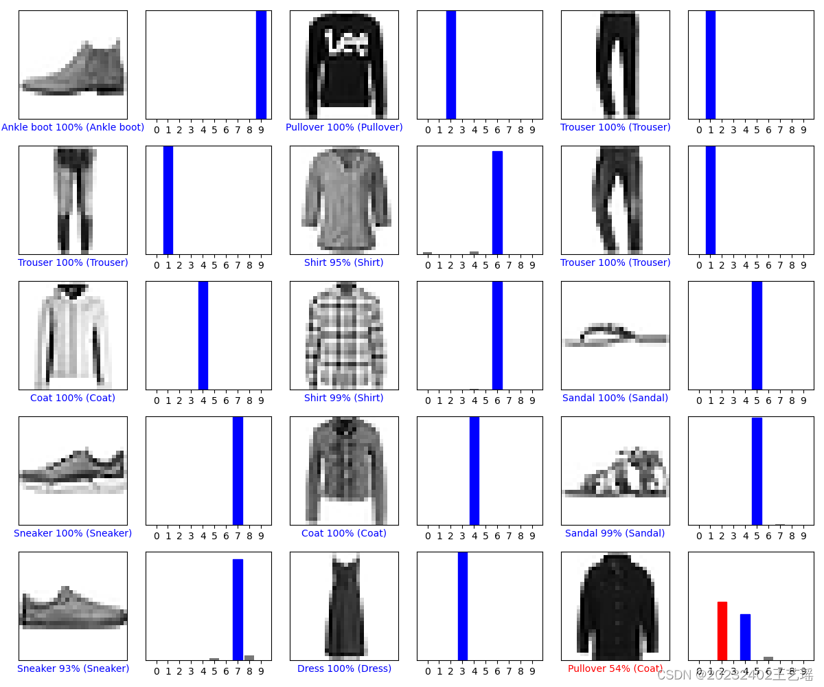
每张图像显示测试集中的一个图像样本，下方标签为预测类别预测置信度% (真实类别)
颜色表示预测的正确性（蓝色表示正确，红色表示错误）
每个条形图显示模型对一个图像的预测概率分布。
x轴表示不同的类别（0-9），y轴表示该类别的预测概率。
灰色的条形表示各个类别的预测概率，红色的条形表示模型的预测类别，蓝色的条形表示真实的类别。

4.2 操作视频

5.源代码

5.1 model.py

import numpy as np
from tensorflow.keras import datasets, layers, models
import matplotlib.pyplot as plt

# 加载Fashion MNIST数据集
(train_images, train_labels), (test_images, test_labels) = datasets.fashion_mnist.load_data()

# 类别名称
name = ['T-shirt/top', 'Trouser', 'Pullover', 'Dress', 'Coat', 'Sandal', 'Shirt', 'trou', 'Bag', 'Ankle boot']

# 图像归一化
train_images = train_images / 255.0
test_images = test_images / 255.0

# 为CNN添加颜色通道
train_images = train_images.reshape((train_images.shape[0], 28, 28, 1))
test_images = test_images.reshape((test_images.shape[0], 28, 28, 1))

# 定义序列模型model
model = (models.Sequential
([
    layers.Conv2D(32, (3, 3), activation='relu', input_shape=(28, 28, 1)),  # 第一层卷积层，Relu激活函数
    layers.MaxPooling2D((2, 2)),  # 最大池化层，降低图的空间尺寸
    layers.Conv2D(64, (3, 3), activation='relu'),  # 第二层卷积层
    layers.MaxPooling2D((2, 2)),
    layers.Flatten(),  # 将多维数据展平为一维，为全连接层做准备
    layers.Dense(64, activation='relu'),  # 全连接层
    layers.Dense(10, activation='softmax')  # 输出层，softmax激活函数输出分类概率分布
]))

# 编译模型
model.compile(optimizer='adam',  # 优化器
              loss='sparse_categorical_crossentropy',  # 损失函数为稀疏分类交叉熵
              metrics=['accuracy'])  # 评估指标为准确率

# 训练模型
history = model.fit(train_images, train_labels,
                    epochs=10,  # 十轮
                    validation_data=(test_images, test_labels))

# 测试
test_loss, test_acc = model.evaluate(test_images, test_labels)
print(f"Test accuracy: {test_acc}")  # f-string 格式化输出

# 绘制训练和测试的准确率曲线
plt.plot(history.history['accuracy'], label='accuracy')  # 训练集准确率曲线
plt.plot(history.history['val_accuracy'], label = 'val_accuracy')  # 测试集
plt.xlabel('Epoch')  # x轴标签
plt.ylabel('Accuracy')
plt.ylim([0, 1])  # y轴的取值范围为0到1
plt.legend(loc='lower right')  # 设置图例显示在右下角
plt.show()

pre = model.predict(test_images)

# 显示图像及其预测结果
def plot_image(i, prearray, trlabel, img):  # 获取第i个样本的预测数组、真实标签和图像
    prearray, trlabel, img = prearray[i], trlabel[i], img[i]
    plt.grid(False)  # 关闭网格
    plt.xticks([])   # 移除x轴刻度
    plt.yticks([])
    plt.imshow(img[...,0], cmap=plt.cm.binary)  # 显示图像，使用二值化颜色映射
    prelabel = np.argmax(prearray)
    if prelabel == trlabel:
        color = 'blue'
    else:
        color = 'red'

    plt.xlabel("{} {:2.0f}% ({})".format(name[prelabel],
                                         100*np.max(prearray),
                                         name[trlabel]),
                                         color=color)   # f-string

# 显示各个类别的预测概率
def plot_value_array(i, prearray, trlabel):
    prearray, trlabel = prearray[i], trlabel[i]
    plt.grid(False)
    plt.xticks(range(10))  # 设置x轴刻度为0-9
    plt.yticks([])
    thisplot = plt.bar(range(10), prearray, color="#777777")  # 绘制条形图，显示每个类别的预测概率，颜色设置为灰色
    plt.ylim([0, 1])
    prelabel = np.argmax(prearray)

    thisplot[prelabel].set_color('red')  # 将预测标签对应的条形图颜色设为红色
    thisplot[trlabel].set_color('blue')  # 将真实标签对应的条形图颜色设为蓝色

# 绘制测试图像及其预测结果
rows = 5  # 图像行数
cols = 3  # 列数
num = rows * cols  # 总数
plt.figure(figsize=(2 * 2 * cols, 2 * rows))  # 创建一个新的图形，设置图形大小
for i in range(num):
    plt.subplot(rows, 2 * cols, 2 * i + 1)
    plot_image(i, pre, test_labels, test_images)
    plt.subplot(rows, 2 * cols, 2 * i + 2)
    plot_value_array(i, pre, test_labels)
plt.tight_layout()
plt.show()

model.save('model.keras')

5.2 classify.py

import tkinter as tk
from tkinter import filedialog, Label
from tkinterdnd2 import DND_FILES, TkinterDnD
from PIL import Image, ImageTk
import numpy as np
from tensorflow.keras.models import load_model
from model import name

# 加载模型
model = load_model('model.keras')


# 图像预处理
def preprocessing(image_path):
    img = Image.open(image_path).convert('L')  # 转换为灰度图像（'L'表示灰度）
    img = img.resize((28, 28))  # 大小调整为28x28像素
    img = np.array(img) / 255.0  # 将图像转换为NumPy数组，并进行归一化处理
    img = img.reshape(1, 28, 28, 1)  # 其中1表示样本数，28x28表示图像大小，1表示通道数（灰度图像只有一个通道）
    return img


# 调整图像大小并保持纵横比
def resize_image(image, new_width, new_height):
    aspect_ratio = image.width / image.height
    if aspect_ratio > 1:  # 宽图像
        new_height = int(new_width / aspect_ratio)
    else:  # 窄图像
        new_width = int(new_height * aspect_ratio)

    resized_image = image.resize((new_width, new_height), Image.LANCZOS)
    return resized_image


# 分类
def classify(image_path):
    img = preprocessing(image_path)
    prediction = model.predict(img)  # 使用模型进行预测
    pre_class = name[np.argmax(prediction)]  # 获取预测的类别

    img_dis = Image.open(image_path)
    img_dis = resize_image(img_dis, 400, 300)  # 调整图像大小为400x300像素
    tk_img = ImageTk.PhotoImage(img_dis)  # 转换成Tkinter格式
    panel.config(image=tk_img)  # 更新Label组件显示的图像
    panel.image = tk_img  # 绑定新的图像对象到Label组件上

    result.config(text=f"Prediction: {pre_class}")  # 更新结果标签


def upload_file():
    file_path = filedialog.askopenfilename()
    if file_path:
        classify(file_path)


def drop(event):
    file_path = event.data
    classify(file_path)


# 创建主窗口
root = TkinterDnD.Tk()
root.title("服装分类")
root.geometry("800x600")

canvas = tk.Canvas(root, width=800, height=600)  # 创建Canvas来放置背景
canvas.pack(fill='both', expand=True)

bg_path = "background.png"
bg = Image.open(bg_path)
bg = resize_image(bg, 800, 600)  # 调整背景图像大小为窗口大小
bg_photo = ImageTk.PhotoImage(bg)
canvas.create_image(0, 0, image=bg_photo, anchor='nw')

frame = tk.Frame(root, bg='white', bd=5)
canvas.create_window(400, 50, window=frame, anchor="n")  # window 参数指定要嵌入到 Canvas 中的窗口小部件

button = tk.Button(frame, text="Upload an image", command=upload_file, font=('Helvetica', 12))  # 按钮
button.grid(row=0, column=0)

result = Label(frame, text="Prediction: ", font=('Helvetica', 14), bg='white')  # 结果标签
result.grid(row=0, column=1)

panel = Label(canvas, bg='white')  # 在Canvas上放置用于显示图像的Label
canvas.create_window(400, 300, window=panel)  # 位置根据需要调整

root.drop_target_register(DND_FILES)  # 绑定拖拽事件
root.dnd_bind('<<Drop>>', drop)

root.mainloop()  # 运行主循环

6. 实验过程中遇到的问题和解决过程

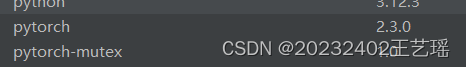
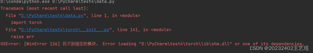
问题1：下载好pytorch后（软件包里已经显示有pytorch了），发现无法找到shm.dll的依赖项
问题1解决方案：
（1）安装Visual C++ 可再发行组件——无果
（2）重新搭建虚拟环境/重新下载pytorch——无果
（3）配置path变量——无果
（4）dependency中查找smh.dll需要的依赖项，发现有一百多个，感到挨个找到并拖到文件夹下有点不太现实。
（5）折腾整整一天后决定使用pytorch的平替TensorFlow（其实也还蛮好用哒~）
问题2：如何获得合适的数据集
问题2解决方案：现爬图片再打标签好像来不及，所以打算找现成的。
开始想做一个可以从衣服图片中提取出衣服风格和场景的模型，打算使用Fashion-Gen Dataset（基于生成对抗网络(GAN)生成的服装图像组成的一个数据集，并附带详细的描述），但这个数据集有点庞大，CPU不太跑得了。所以改为识别衣服类型，使用Fashion-MNIST数据集来实现。
问题3：UserWarning: Glyph 30701 (\N{CJK UNIFIED IDEOGRAPH-77ED}) missing from current font.缺乏中文字体
问题3解决方案：改用英文即可
问题4：生成界面的图片长宽比例被改变了，有点小丑

原图如下：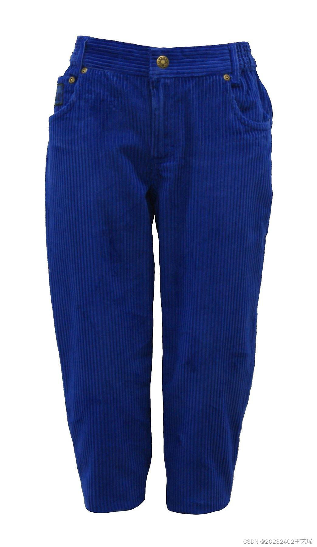
问题4解决方案：

# 调整图像大小并保持纵横比
def resize_image(image, target_width, target_height):
    aspect_ratio = image.width / image.height
    if target_width / target_height > aspect_ratio:
        new_height = target_height
        new_width = int(aspect_ratio * target_height)
    else:
        new_width = target_width
        new_height = int(target_width / aspect_ratio)

    return image.resize((new_width, new_height), Image.LANCZOS)

Image.ANTIALIAS不能用，可换成Image.LANCZOS

问题5：写交互界面时不断出现背景盖过图片和检测结果、背景和边框搭配不协调等问题。
问题5解决方案：使用Canvas。Canvas 是一个灵活强大的绘图区域，可以绘制图形和图像，并且可以在其上放置其他组件。把frame 嵌入到 canvas 中，作为一个容器来放置按钮和标签，可以使布局更整齐。

7.实验感想体会

因为准备做关于虚拟试衣课题的大创，之前学过一点深度学习/机器学习和pytorch，但一直是理论学习，并未实践过。正好想借此机会尝试一下训练一个简单的模型。
这次实验是一口气做完的，搭环境一天，编程序+调代码+写报告用了14h。这期间先是经历了pytorch无论如何跑不通，问大模型、问研究生学长、问做软件的亲戚、问娄老师，大家都没有好的解决办法。这24h我过得极其沮丧和崩溃，有种浪费了时间没有成果的挫败感。好在后来下载tensorflow.keras十分顺利，柳暗花明又一村。环境搭好之后就开始马不停蹄地编程。从5月29日15:30到5月30日6:00,除了听党课1h，剩下的13个半小时，一直坐在电脑前写程序，看着身边窗外的太阳落下又升起，我却全然感受不到时间的流逝。因为编程实在是太有意思了，python更是，人工智能更是，看着我敲出的代码所生成的成果，虽然简陋，但却是从未有过新奇体验；虽然过程艰辛，但代码跑通的一刻喜悦之情难以言表。

全课总结

经过这一个学期的python学习，我对python的语法、python多种多样的库、面向对象的程序设计以及python所能实现的各种各样有趣的功能（如游戏、爬虫、数据处理、可视化、机器学习、神经网络等）有了初步的了解，深刻体会到了python的趣味性与实用性。
志强老师真的是我见过的最好的那种老师，温柔善良、耐心亲和、活泼幽默，而且会给我们提供很多中肯且宝贵的建议。最令我印象深刻的是最后一节课上老师的寄语，“如果你觉得你没有高三那么努力了，那就要注意了”，以及“功不唐捐，玉汝于成”。志强老师说早八前的20分钟和上午大课间的20分钟是要充分利用的，我也曾见过志强老师深夜十二点多在办公室里为学生解答问题，志强老师的言传身教让我明白，优秀的人更努力。曾经我也许会怀疑在我们学校拼命学习的重要性，但现在我觉得，认真是一种态度，拼搏是一种习惯，每一个不曾起舞的日子都是对生命的辜负。
在这里插入图片描述

另外，志强老师强调不要过度依赖大模型，我觉得确实如此。现如今，人工智能发展迅猛，如何学会利用它帮助提升自己、提高自学效率，而不是让AI代替我们学习，成为了重要的课题。本次实验的很多内容都借助了大模型的帮助，但代码我一定会自己敲一遍，尽可能理解它们的意思，化大模型的知识为自己的知识。
最后再次感谢与python公选课的相遇、与志强老师的相遇，受益匪浅、收获颇丰。

参考资料

《PyTorch深度学习笔记（7）：应用实例–FashionMNIST数据集》

20232402王艺瑶

关注

35
点赞
踩
10

收藏

觉得还不错? 一键收藏
1
评论
20232402 2023-2024-2 《Python程序设计》实验四报告

经过这一个学期的python学习，我对python的语法、python多种多样的库、面向对象的程序设计以及python所能实现的各种各样有趣的功能（如游戏、爬虫、数据处理、可视化、机器学习、神经网络等）有了初步的了解，深刻体会到了python的趣味性与实用性。志强老师真的是我见过的最好的那种老师，温柔善良、耐心亲和、活泼幽默，而且会给我们提供很多中肯且宝贵的建议。最令我印象深刻的是最后一节课上老师的寄语，“如果你觉得你没有高三那么努力了，那就要注意了”，以及“功不唐捐，玉汝于成”。
复制链接

扫一扫