


1. Pandas
1.1 pd.loc & pd.iloc 取出多行多列数据
loc函数主要通过行标签进行索引
iloc函数主要通过列标签进行索引
data :
    A   B   C   D
a   0   1   2   3
b   4   5   6   7
c   8   9  10  11
d  12  13  14  15

# 取索引为'a'的行
data.loc['a']

# 取第一行数据,索引为'a'的行就是第一行,所以结果相同
data.iloc[0]

# 取列数据
data.loc[:,'A']
data.iloc[:,[0]]

# 取多行多列

#提取index为'a','b',列名为'A','B'中的数据
data.loc[['a','b'],['A','B']]

#提取第0、1行,第0、1列中的数据
data.iloc[[0,1],[0,1]]

# 根据条件筛选数据行

# 筛选条件: A列中数字为0所在的行数据或B列中数字为0所在的行数据
data.loc[(data['A']==0)|(data['B']==2)]
可以发现loc是通过index的具体特征来提取数据
而iloc是通过index的第几行第几列来提取特征
1.2 pd.at 通过行列标签取出单个数据
# 第一行,列标签为a的数据
data.at[0, 'a']
1.3 pd.isnull() 返回二值数组判断是否为NaN
nan_all = data.isnull()
print(nan_all)
    col1   col2   col3   col4
0  False  False  False  False
1  False   True  False  False
2  False  False  False  False
3  False  False  False  False
4  False  False  False   True
5  False  False  False  False

# print(nan_all.any()) # 获得含有缺失值的列
# print(nan_all.all()) # 获得全部都是缺失值的列
1.4 pd.dropna() 直接丢弃含有NA的行记录
data.dropna()
1.5 pd.fillna() 填充缺失值
# 常数填充
data.fillna(100)

# 通过字典填充
data.fillna({0:10,2:20}) # 第0列的缺失值使用10来填充,第二列的缺失值使用20填充

# 通过method方法填充
data.fillna(method='ffill/bfill', limit=2) #用前/后一个值填充 limit限制填充个数

# 默认按照行的方式填充 通过参数axis=1改为列填充

data.fillna({'col2': 1.1, 'col4': 1.2})  # 用不同值替换不同列的缺失值
data.fillna(data.mean()['col2':'col4'])  # 用平均数代替,选择各自列的均值替换缺失值
1.6 pd.duplicated()重复值处理
# 打印判断重复数据记录(true/false)
print(data.duplicated())

# 删除重复值
print(df.drop_duplicates())  # 删除数据记录中所有行值相同的记录
print(df.drop_duplicates(['col1']))  # 删除数据记录中col1值相同的记录
print(df.drop_duplicates(['col1', 'col2']))  # 除数据记录中指定列(col1/col2)值相同的记录
1.7 通过pd[[col]]直接获取col列标签所在的数据列
id_data = df[['id']] # 获得ID列
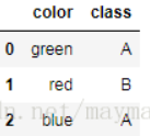
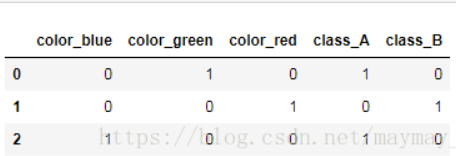
1.8 pd.get_dummies()实现独热编码
# 函数原型
pandas.get_dummies(data, prefix=None, prefix_sep='_', dummy_na=False, columns=None, sparse=False, drop_first=False)


df = pd.DataFrame([
            ['green' , 'A'],
            ['red'   , 'B'],
            ['blue'  , 'A']])
pd.get_dummies(df)
1.9 pd.concat()连接函数
函数原型
pd.concat(objs, axis=0, join='outer', join_axes=None, ignore_index=False,
          keys=None, levels=None, names=None, verify_integrity=False,
          copy=True)

axis : 0为行连接 1为列连接
key : 识别数据源原来属于哪个dataframe
join : 分为inner表的交集和outer表的并集
objs :需要合并的表可以使用元组或者列表() [ ]

frames = [df1, df2, df3]

result = pd.concat(frames)
1.10 train_test_split
from sklearn.model_selection import train_test_split

x_train,x_test, y_train, y_test = train_test_split(X, y, test_size=0.3, random_state=0) # test_size=.3表示测试集占70%
2. Numpy
2.1 np.loadtxt(filename, dtype, delimiter)
np.loadtxt('name.txt', dtype='float32', delimiter=' ') # 最后一个参数是分隔符
2.2 np.save(file_name, data)
write_data = np.array([[1, 2, 3, 4], [5, 6, 7, 8], [9, 10, 11, 12]])
np.save('load_data', write_data)
# 注意这里保存的是.npy文件格式
# 第一个参数是文件的名字,第二个参数是需要导入的数据——需要是array格式
2.3 np.load(filename)
read_data = np.load('load_data.npy')  # 读取npy文件
print(read_data)  # 输出读取的数据
2.4 np.split()划分数据集
使用pandas中的train_test_split()无法划分除了常规的4部分以外的划分比如训练集,测试集,验证集
split(ary, indices_or_sections, axis=0)
ary : 原始数据集
indices_or_sections : 一个整型数K(均分为K份);一个一维数组(按给出数量划分)

import numpy as np
x = np.arange(72).reshape((24, 3)) # 创建24行3列的数组
train, test, val = np.split(x, 3) # 均分为三份
train, test, val = np.split(x, [int(0.6*x.shape[0]), int(0.9*x.shape[0])]) # 60% 30% 10%
3. Sklearn
3.1 生成模型的三个步骤
model = LinearRession() 将模型实例化(括号中可以选填参数)
model = fit.(x_train, y_train) 将训练集导入fit
pre_y = model.predict(x_test) 通过model中的方法predict来预测结果
3.2 注意sklearn中的所有数据都必须是array
.reshape[-1, 1]
3.3 Imputer填充空值
from sklearn.impute import SimpleImputer
# 使用sklearn将缺失值替换为特定值

nan_model = SimpleImputer(strategy="most_frequent")  # 建立替换规则:将值为NaN的缺失值以众数做替换
nan_result = nan_model.fit_transform(df)  # 应用模型规则
print(nan_result)  # 打印输出
# 一般对于pandas这种带有标签的填充,我们的strategy使用constant或者most_frequent
3.4 OneHotEncoder独热编码
from sklearn.preprocessing import OneHotEncoder # 导入库
# 原始数据
        id     sex   level  score
0  3566841    male    high      1
1  6541227  Female     low      2
2  3512441  Female  middle      3

# 拆分ID和数据列
id_data = df[['id']]  # 获得ID列
raw_convert_data = df.iloc[:, 1:]  # 取出后三列
print(raw_convert_data) # 打印

model = OneHotEncoder()  # 建立标志转换模型对象(也称为哑编码对象)
new = model.fit_transform(raw_convert_data).toarray()  # 标志转换
# 合并数据
df_all = pd.concat((id_data, pd.DataFrame(df_new2)), axis=1)  # 重新组合为数据框
print(df_all)  # 打印输出转换后的数据框

      sex   level  score
0    male    high      1
1  Female     low      2
2  Female  middle      3

        id    0    1    2    3    4    5    6    7
0  3566841  0.0  1.0  1.0  0.0  0.0  1.0  0.0  0.0
1  6541227  1.0  0.0  0.0  1.0  0.0  0.0  1.0  0.0
2  3512441  1.0  0.0  0.0  0.0  1.0  0.0  0.0  1.0
3.5 feature_selection特征选择
Scikit-learn 将特征选择的内容作为实现了 transform 方法的对象
1. 移除低方差特征
from sklearn.feature_selection import VarianceThreshold
sel = VarianceThreshold(threshold=0.5) # 将方差低于0.5的特征列移除
sel.fit_transform(x_train)

2. 单变量特征选择
单独计算每个变量的某个统计指标,根据该指标来判断哪些指标重要
SelectKBest 移除得分前 k 名以外的所有特征(取top k)
SelectPercentile 移除得分在用户指定百分比以后的特征(取top k%)

from sklearn import feature_selection
sel = feature_selection.SelectKBest() # 加上参数k=?得到前几
sel_2 = feature_selection.SelectPercentile(percentile=30) # 取前30%得分的特征
这里我们还可以调整选择的策略
对于分类问题(y值离散)
卡方验证(chi2)
f_classif
mutual_info_classif

对于回归问题(y值连续)
f_regression
mutual_info_regression
3.6 标准化——让数据落入相同的区间
import numpy as np
from sklearn import preprocessing # 导入预处理库

# Z-Score标准化
zscore_scaler = preprocessing.StandardScaler()  # 建立StandardScaler对象

# Max-Min标准化
minmax_scaler = preprocessing.MinMaxScaler()  # 建立MinMaxScaler模型对象

# MaxAbsScaler标准化
maxabsscaler_scaler = preprocessing.MaxAbsScaler()  # 建立MaxAbsScaler对象

# RobustScaler标准化
robustscalerr_scaler = preprocessing.RobustScaler()  # 建立RobustScaler标准化对象
3.7 PMMLpython与其他程序环境的模型交互
pip install sklearn2pmml #按照相关类库

from sklearn2pmml.pipeline import PMMLPipeline
from sklearn2pmml import sklearn2pmml

# 构造pipe
pipeline = PMMLPipeline([("kmeans",
						  KMeans(n_clusters=n_clusters,
						  random_state=0))])
pipeline.fit(data)

# 导出对象
sklearn2pmml(pipeline, "kmeans.pmml", with_repr = True)
3.8 imblearn——解决数据不均衡问题
3.8.1 过采样
1. 通过从少数类的样本中进行随机采样来增加新的样本
from imblearn.over_sampling import RandomOverSampler

ros = RandomOverSampler(random_state=0)
X_resampled, y_resampled = ros.fit_sample(X, y)
2. SMOTE: 对于少数类样本a, 随机选择一个最近邻的样本b, 然后从a与b的连线上随机选取一个点c作为新的少数类样本
3. ADASYN: 关注的是在那些基于K最近邻分类器被错误分类的原始样本附近生成新的少数类样本
from imblearn.over_sampling import SMOTE, ADASYN

X_resampled_smote, y_resampled_smote = SMOTE().fit_sample(X, y)
X_resampled_adasyn, y_resampled_adasyn = ADASYN().fit_sample(X, y)
3.8.2 欠采样
1. 原型生成:原型生成方法将减少数据集的样本数量, 剩下的样本是由原始数据集生成的, 而不是直接来源于原始数据集

ClusterCentroids函数:每一个类别的样本都会用K-Means算法的中心点来进行合成, 而不是随机从原始样本进行抽取
from imblearn.under_sampling import ClusterCentroids

cc = ClusterCentroids(random_state=0)
X_resampled, y_resampled = cc.fit_sample(X, y)
2. 原型选择
2.1 RandomUnderSampler函数:随机选取数据的子集

from imblearn.under_sampling import RandomUnderSampler

rus = RandomUnderSampler(random_state=0)
X_resampled, y_resampled = rus.fit_sample(X, y)

2.2 NearMiss函数:添加了一些启发式(heuristic)的规则来选择样本, 通过设定version参数来实现三种启发式的规则

from imblearn.under_sampling import NearMiss

nm1 = NearMiss(random_state=0, version=1)
X_resampled_nm1, y_resampled = nm1.fit_sample(X, y)

NearMiss-1: 选择离N个近邻的负样本的平均距离最小的正样本;

NearMiss-2: 选择离N个负样本最远的平均距离最小的正样本;

NearMiss-3: 是一个两段式的算法. 首先, 对于每一个负样本, 保留它们的M个近邻样本; 接着, 那些到N个近邻样本平均距离最大的正样本将被选择.

2.3 EditedNearestNeighbours函数:这种方法应用最近邻算法来编辑(edit)数据集, 找出那些与邻居不太友好的样本然后移除. 对于每一个要进行下采样的样本, 那些不满足一些准则的样本将会被移除
from imblearn.under_sampling import EditedNearestNeighbours
from imblearn.under_sampling import RepeatedEditedNearestNeighbours(将该算法重复多次)

2.4 ALLKNN算法:进行每次迭代的时候, 最近邻的数量都在增加
from imblearn.under_sampling import AllKNN
3.8.3 过采样和欠采样的结合
由边界的样本与其他样本进行过采样差值时, 很容易生成一些噪音数据. 因此, 在过采样之后需要对样本进行清洗。 所以就有了两种结合过采样与下采样的方法: (i) SMOTETomek and (ii) SMOTEENN
from imblearn.combine import SMOTEENN
smote_enn = SMOTEENN(random_state=0)
X_resampled, y_resampled = smote_enn.fit_sample(X, y)

from imblearn.combine import SMOTETomek
smote_tomek = SMOTETomek(random_state=0)
X_resampled, y_resampled = smote_tomek.fit_sample(X, y)
3.8.4 Ensemble
通过多个均衡的子集来实现不均衡集合的均衡化
1. EasyEnsemble:通过对原始的数据集进行随机下采样实现对数据集进行集成
from imblearn.ensemble import EasyEnsemble

ee = EasyEnsemble(random_state=0, n_subsets=10, replacement=True)
# n_subsets控制子集的数量、replacement控制是否放回抽样
X_resampled, y_resampled = ee.fit_sample(X, y)
2. BalanceCascade(级联平衡):通过使用分类器(estimator参数)来确保那些被错分类的样本在下一次进行子集选取的时候也能被采样到

from imblearn.ensemble import BalanceCascade
from sklearn.linear_model import LogisticRegression
bc = BalanceCascade(random_state=0,
                    estimator=LogisticRegression(random_state=0),
                    n_max_subset=4 # 最大子集数)
X_resampled, y_resampled = bc.fit_sample(X, y)
3. BalancedBaggingClassifier:允许在训练每个基学习器之前对每个子集进行重抽样. 简而言之, 该方法结合了EasyEnsemble 采样器与分类器(如BaggingClassifier)的结果
4.
from imblearn.ensemble import BalancedBaggingClassifier
bbc = BalancedBaggingClassifier(base_estimator=DecisionTreeClassifier(),
                                ratio='auto',
                                replacement=False,
                                random_state=0)
bbc.fit(X, y)
y_pred = bbc.predict(X_test)
3.9 confusion_matrix()混淆矩阵——分类评估
sklearn.metrics.confusion_matrix(y_true, y_pred, labels=None, sample_weight=None)

y_true: 是样本真实分类结果
y_pred: 是样本预测分类结果
labels:对类别进行选择
sample_weight : 样本权重


# 二分类混淆矩阵
tn, fp, fn, tp = confusion_matrix(y_test, pre_y).ravel()
# .raevl 将多维矩阵平铺为一维
# 获得混淆矩阵
3.10 XGBoost输出特征重要性
需要导入Matplotlib库
import xgboost as xgb
import matplotlib.pyplot as plt

# XGB分类模型训练
param_dist = {'objective': 'binary:logistic', 'n_estimators': 10,
              'subsample': 0.8, 'max_depth': 10, 'n_jobs': -1}
model_xgb = xgb.XGBClassifier(**param_dist)
model_xgb.fit(X_train, y_train)
pre_y = model_xgb.predict(X_test)

xgb.plot_importance(model, height=0.5, importance_type='gain',
					max_num_features=10, xlabel='Gain Split',
					grid=False)
model : 树模型对象
height : 条形图的高度
importance_type : 特征重要度的计算分为:
					weight :特征在树中的出现次数
					gain :使用该特征的平均增益值
					cover :使用作为分裂节点的覆盖的样本比例
grid :设置为false不显示网格线

# 输出树形规则图
xgb.to_graphviz(model_xgb, num_trees=1, yes_color='#638e5e', no_color='#a40000')
4. Tensorflow
5. Opencv
5.1 cv2.imread()读取图片
#!pip install https://download.lfd.uci.edu/pythonlibs/h2ufg7oq/opencv_python-3.4.3-cp37-cp37m-win_amd64.whl
import cv2  # 导入库
file = 'cat.jpg'  # 定义图片地址
img = cv2.imread(file)  # 读取图像
cv2.imshow('image', img)  # 展示图像
5.2 cv2.VideoCapture()获得视频对象
import cv2  # 导入库
cap = cv2.VideoCapture("tree.avi")  # 获得视频对象
status = cap.isOpened()  # 判断文件是否正确打开
# 读取视频内容并展示视频
success, frame = cap.read()  # 读取视频第一帧
while success:  # 如果读取状态为True
    cv2.imshow('vidoe frame', frame)  # 展示帧图像
    success, frame = cap.read()  # 获取下一帧
    k = cv2.waitKey(int(1000 / frame_fps))  # 每次帧播放延迟一定时间,同时等待输入指令
    if k == 27:  # 如果等待期间检测到按键ESC
        break  # 退出循环

# 操作结束释放所有对象
cv2.destroyAllWindows()  # 关闭所有窗口
cap.release()  # 释放视频文件对象


 736
736


 被折叠的 条评论
为什么被折叠?
被折叠的 条评论
为什么被折叠?
 到【灌水乐园】发言


