


1. SIFT: Introduction
Matching features across different images in a common problem in computer vision. When all images are similar in nature (same scale, orientation, etc) simple corner detectors can work. But when you have images of different scales and rotations, you need to use the Scale Invariant Feature Transform.
Why care about SIFT
SIFT isn't just scale invariant. You can change the following, and still get good results:
- Scale (duh)
- Rotation
- Illumination
- Viewpoint
Here's an example. We're looking for these:

And we want to find these objects in this scene:

Here's the result:

Now that's some real robust image matching going on. The big rectangles mark matched images. The smaller squares are for individual features in those regions. Note how the big rectangles are skewed. They follow the orientation and perspective of the object in the scene.
The algorithm
SIFT is quite an involved algorithm. It has a lot going on and can become confusing, So I've split up the entire algorithm into multiple parts. Here's an outline of what happens in SIFT.
- Constructing a scale space This is the initial preparation. You create internal representations of the original image to ensure scale invariance. This is done by generating a "scale space".
- LoG Approximation The Laplacian of Gaussian is great for finding interesting points (or key points) in an image. But it's computationally expensive. So we cheat and approximate it using the representation created earlier.
- Finding keypoints With the super fast approximation, we now try to find key points. These are maxima and minima in the Difference of Gaussian image we calculate in step 2
- Get rid of bad key points Edges and low contrast regions are bad keypoints. Eliminating these makes the algorithm efficient and robust. A technique similar to the Harris Corner Detector is used here.
- Assigning an orientation to the keypoints An orientation is calculated for each key point. Any further calculations are done relative to this orientation. This effectively cancels out the effect of orientation, making it rotation invariant.
- Generate SIFT features Finally, with scale and rotation invariance in place, one more representation is generated. This helps uniquely identify features. Lets say you have 50,000 features. With this representation, you can easily identify the feature you're looking for (say, a particular eye, or a sign board). That was an overview of the entire algorithm. Over the next few days, I'll go through each step in detail. Finally, I'll show you how to implement SIFT in OpenCV!
What do I do with SIFT features?
After you run through the algorithm, you'll have SIFT features for your image. Once you have these, you can do whatever you want.
Track images, detect and identify objects (which can be partly hidden as well), or whatever you can think of. We'll get into this later as well.
But the catch is, this algorithm is patented.
.<
So, it's good enough for academic purposes. But if you're looking to make something commercial, look for something else! [Thanks to aLu for pointing out SURF is patented too]
2. SIFT: The scale space
Real world objects are meaningful only at a certain scale. You might see a sugar cube perfectly on a table. But if looking at the entire milky way, then it simply does not exist. This multi-scale nature of objects is quite common in nature. And a scale space attempts to replicate this concept on digital images.
Scale spaces
Do you want to look at a leaf or the entire tree? If it's a tree, get rid of some detail from the image (like the leaves, twigs, etc) intentionally.
While getting rid of these details, you must ensure that you do not introduce new false details. The only way to do that is with the Gaussian Blur (it was proved mathematically, under several reasonable assumptions).
So to create a scale space, you take the original image and generate progressively blurred out images. Here's an example:

Look at how the cat's helmet loses detail. So do it's whiskers.
Scale spaces in SIFT
SIFT takes scale spaces to the next level. You take the original image, and generate progressively blurred out images. Then, you resize the original image to half size. And you generate blurred out images again. And you keep repeating.
Here's what it would look like in SIFT:
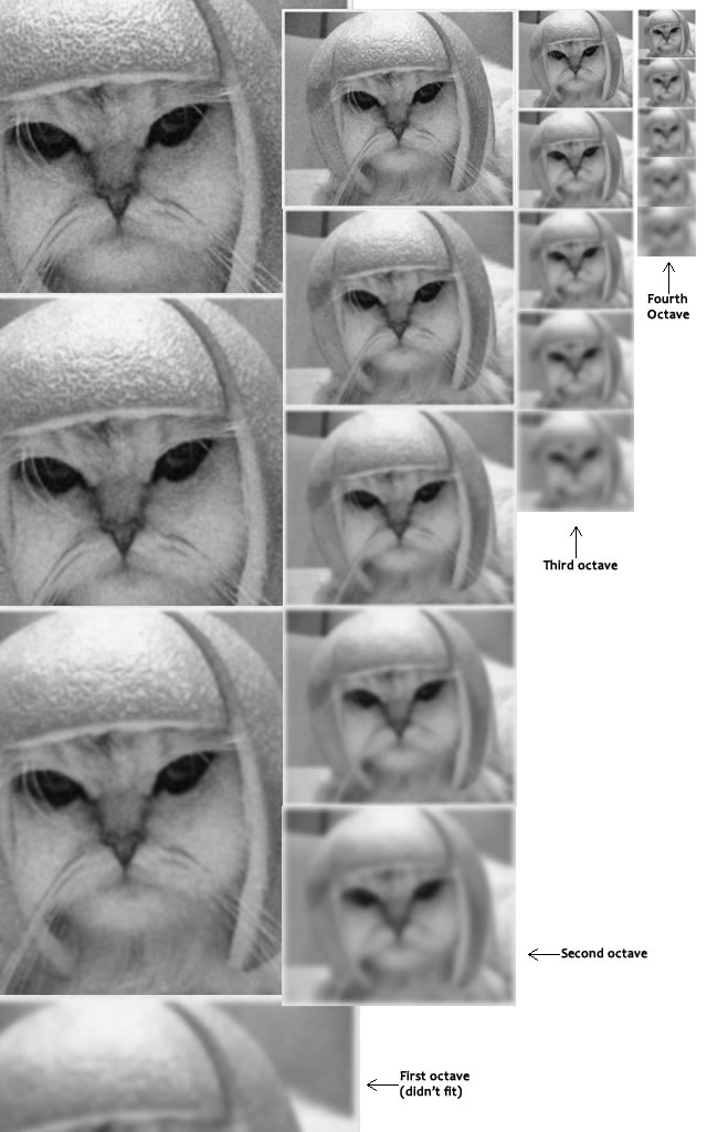
Images of the same size (vertical) form an octave. Above are four octaves. Each octave has 5 images. The individual images are formed because of the increasing "scale" (the amount of blur).
The technical details
Now that you know things the intuitive way, I'll get into a few technical details.
Octaves and Scales
The number of octaves and scale depends on the size of the original image. While programming SIFT, you'll have to decide for yourself how many octaves and scales you want. However, the creator of SIFT suggests that 4 octaves and 5 blur levels are ideal for the algorithm.
The first octave
If the original image is doubled in size and antialiased a bit (by blurring it) then the algorithm produces more four times more keypoints. The more the keypoints, the better!
Blurring
Mathematically, "blurring" is referred to as the convolution of the gaussian operator and the image. Gaussian blur has a particular expression or "operator" that is applied to each pixel. What results is the blurred image.

The symbols:
- L is a blurred image
- G is the Gaussian Blur operator
- I is an image
- x,y are the location coordinates
- σ is the "scale" parameter. Think of it as the amount of blur. Greater the value, greater the blur.
- The * is the convolution operation in x and y. It "applies" gaussian blur G onto the image I.

This is the actual Gaussian Blur operator.
Amount of blurring
The amount of blurring in each image is important. It goes like this. Assume the amount of blur in a particular image is σ. Then, the amount of blur in the next image will be k*σ. Here k is whatever constant you choose.

This is a table of σ's for my current example. See how each σ differs by a factor sqrt(2) from the previous one.
Summary
In the first step of SIFT, you generate several octaves of the original image. Each octave's image size is half the previous one. Within an octave, images are progressively blurred using the Gaussian Blur operator.
In the next step, we'll use all these octaves to generate Difference of Gaussian images.
3. SIFT: LoG approximations
In the previous step , we created the scale space of the image. The idea was to blur an image progressively, shrink it, blur the small image progressively and so on. Now we use those blurred images to generate another set of images, the Difference of Gaussians (DoG). These DoG images are a great for finding out interesting key points in the image.
Laplacian of Gaussian
The Laplacian of Gaussian (LoG) operation goes like this. You take an image, and blur it a little. And then, you calculate second order derivatives on it (or, the "laplacian"). This locates edges and corners on the image. These edges and corners are good for finding keypoints.
But the second order derivative is extremely sensitive to noise. The blur smoothes it out the noise and stabilizes the second order derivative.
The problem is, calculating all those second order derivatives is computationally intensive. So we cheat a bit.
The Con
To generate Laplacian of Guassian images quickly, we use the scale space. We calculate the difference between two consecutive scales. Or, the Difference of Gaussians. Here's how:
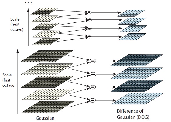
These Difference of Gaussian images are approximately equivalent to the Laplacian of Gaussian. And we've replaced a computationally intensive process with a simple subtraction (fast and efficient). Awesome!
These DoG images comes with another little goodie. These approximations are also "scale invariant". What does that mean?
The Benefits
Just the Laplacian of Gaussian images aren't great. They are not scale invariant. That is, they depend on the amount of blur you do. This is because of the Gaussian expression. (Don't panic ;) )
See the σ2 in the demonimator? That's the scale. If we somehow get rid of it, we'll have true scale independence. So, if the laplacian of a gaussian is represented like this:

Then the scale invariant laplacian of gaussian would look like this:

But all these complexities are taken care of by the Difference of Gaussian operation. The resultant images after the DoG operation are already multiplied by the σ2. Great eh!
Oh! And it has also been proved that this scale invariant thingy produces much better trackable points! Even better!
Side effects
You can't have benefits without side effects >.<
You know the DoG result is multiplied with σ2. But it's also multiplied by another number. That number is (k-1). This is the k we discussed in the previous step.
But we'll just be looking for the location of the maximums and minimums in the images. We'll never check the actual values at those locations. So, this additional factor won't be a problem to us. (Even if you multiply throughout by some constant, the maxima and minima stay at the same location)
Example
Here's a gigantic image to demonstrate how this difference of Gaussians works.

In the image, I've done the subtraction for just one octave. The same thing is done for all octaves. This generates DoG images of multiple sizes.
Summary
Two consecutive images in an octave are picked and one is subtracted from the other. Then the next consecutive pair is taken, and the process repeats. This is done for all octaves. The resulting images are an approximation of scale invariant laplacian of gaussian (which is good for detecting keypoints). There are a few "drawbacks" due to the approximation, but they won't affect the algorithm.
Next, we'll actually find some interesting keypoints. Maxima and Minima. Or, Maximums and Minimums of the image.
4. SIFT: Finding keypoints
Up till now, we have generated a scale space and used the scale space to calculate the Difference of Gaussians. Those are then used to calculate Laplacian of Gaussian approximations that is scale invariant. I told you that they produce great key points. Here's how it's done!
Finding key points is a two part process
- Locate maxima/minima in DoG images
- Find subpixel maxima/minima
Locate maxima/minima in DoG images
The first step is to coarsely locate the maxima and minima. This is simple. You iterate through each pixel and check all it's neighbours. The check is done within the current image, and also the one above and below it. Something like this:
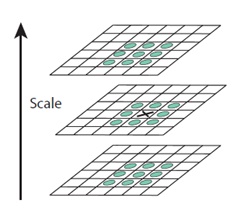
X marks the current pixel. The green circles mark the neighbours. This way, a total of 26 checks are made. X is marked as a "key point" if it is the greatest or least of all 26 neighbours.
Usually, a non-maxima or non-minima position won't have to go through all 26 checks. A few initial checks will usually sufficient to discard it.
Note that keypoints are not detected in the lowermost and topmost scales. There simply aren't enough neighbours to do the comparison. So simply skip them!
Once this is done, the marked points are the approximate maxima and minima. They are "approximate" because the maxima/minima almost never lies exactly on a pixel. It lies somewhere between the pixel. But we simply cannot access data "between" pixels. So, we must mathematically locate the subpixel location.
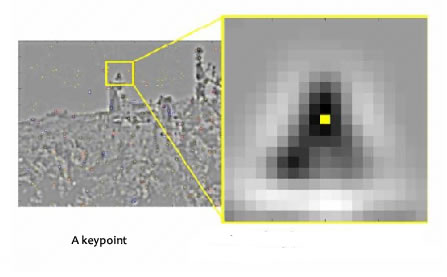
Here's what I mean:
![]()
The red crosses mark pixels in the image. But the actual extreme point is the green one.
Find subpixel maxima/minima
Using the available pixel data, subpixel values are generated. This is done by the Taylor expansion of the image around the approximate key point.
Mathematically, it's like this:

We can easily find the extreme points of this equation (differentiate and equate to zero). On solving, we'll get subpixel key point locations. These subpixel values increase chances of matching and stability of the algorithm.
Example
Here's a result I got from the example image I've been using till now:
 The author of SIFT recommends generating two such extrema images. So, you need exactly 4 DoG images. To generate 4 DoG images, you need 5 Gaussian blurred images. Hence the 5 level of blurs in each octave.
In the image, I've shown just one octave. This is done for all octaves. Also, this image just shows the first part of keypoint detection. The Taylor series part has been skipped.
Summary
Here, we detected the maxima and minima in the DoG images generated in the previous step. This is done by comparing neighbouring pixels in the current scale, the scale "above" and the scale "below".
Next, we'll reject some keypoints detected here. This is because they either don't have enough contrast or they lie on an edge
5. SIFT: Getting rid of low contrast keypoints
Key points generated in the previous step produce a lot of key points. Some of them lie along an edge, or they don't have enough contrast. In both cases, they are not useful as features. So we get rid of them. The approach is similar to the one used in the Harris Corner Detector for removing edge features. For low contrast features, we simply check their intensities.
Removing low contrast features
This is simple. If the magnitude of the intensity (i.e., without sign) at the current pixel in the DoG image (that is being checked for minima/maxima) is less than a certain value, it is rejected.
Because we have subpixel keypoints (we used the Taylor expansion to refine keypoints), we again need to use the taylor expansion to get the intensity value at subpixel locations. If it's magnitude is less than a certain value, we reject the keypoint.
Removing edges
The idea is to calculate two gradients at the keypoint. Both perpendicular to each other. Based on the image around the keypoint, three possibilities exist. The image around the keypoint can be:
- A flat region: If this is the case, both gradients will be small.
- An edge: Here, one gradient will be big (perpendicular to the edge) and the other will be small (along the edge)
- A "corner": Here, both gradients will be big.
Corners are great keypoints. So we want just corners. If both gradients are big enough, we let it pass as a key point. Otherwise, it is rejected.
Mathematically, this is achieved by the Hessian Matrix. Using this matrix, you can easily check if a point is a corner or not.
If you're interested in the math, first check the posts on the Harris corner detector. A lot of the same math used used in SIFT. In the Harris Corner Detector, two eigenvalues are calculated. In SIFT, efficiency is increased by just calculating the ratio of these two eigenvalues. You never need to calculate the actual eigenvalues.
Example
Here's a visual example of what happens in this step:
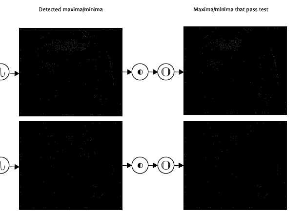
Both extrema images go through the two tests: the contrast test and the edge test. They reject a few keypoints (sometimes a lot) and thus, we're left with a lower number of keypoints to deal with.
Summary
In this step, the number of keypoints was reduced. This helps increase efficiency and also the robustness of the algorithm. Keypoints are rejected if they had a low contrast or if they were located on an edge.
In the next step we'll assign an orientation to all the keypoints that passed both tests.
6. SIFT: Keypoint orientations
After step 4, we have legitimate key points. They've been tested to be stable. We already know the scale at which the keypoint was detected (it's the same as the scale of the blurred image). So we have scale invariance. The next thing is to assign an orientation to each keypoint. This orientation provides rotation invariance. The more invariance you have the better it is. :P
The idea
The idea is to collect gradient directions and magnitudes around each keypoint. Then we figure out the most prominent orientation(s) in that region. And we assign this orientation(s) to the keypoint.
Any later calculations are done relative to this orientation. This ensures rotation invariance.
The size of the "orientation collection region" around the keypoint depends on it's scale. The bigger the scale, the bigger the collection region.
The details
Now for the little details about collecting orientations.

Gradient magnitudes and orientations are calculated using these formulae:

The magnitude and orientation is calculated for all pixels around the keypoint. Then, A histogram is created for this.
In this histogram, the 360 degrees of orientation are broken into 36 bins (each 10 degrees). Lets say the gradient direction at a certain point (in the "orientation collection region") is 18.759 degrees, then it will go into the 10-19 degree bin. And the "amount" that is added to the bin is proportional to the magnitude of gradient at that point.
Once you've done this for all pixels around the keypoint, the histogram will have a peak at some point.
Above, you see the histogram peaks at 20-29 degrees. So, the keypoint is assigned orientation 3 (the third bin)
Also, any peaks above 80% of the highest peak are converted into a new keypoint. This new keypoint has the same location and scale as the original. But it's orientation is equal to the other peak.
So, orientation can split up one keypoint into multiple keypoints.

The Technical Details
Magnitudes
Saw the gradient magnitude image above? In SIFT, you need to blur it by an amount of 1.5*sigma.
Size of the window
The window size, or the "orientation collection region", is equal to the size of the kernel for Gaussian Blur of amount 1.5*sigma.
Summary
To assign an orientation we use a histogram and a small region around it. Using the histogram, the most prominent gradient orientation(s) are identified. If there is only one peak, it is assigned to the keypoint. If there are multiple peaks above the 80% mark, they are all converted into a new keypoint (with their respective orientations).
Next, we generate a highly distinctive "fingerprint" for each keypoint. Here's a little teaser. This fingerprint, or "feature vector", has 128 different numbers.
7. SIFT: Generating a feature
Now for the final step of SIFT. Till now, we had scale and rotation invariance. Now we create a fingerprint for each keypoint. This is to identify a keypoint. If an eye is a keypoint, then using this fingerprint, we'll be able to distinguish it from other keypoints, like ears, noses, fingers, etc.
The idea
We want to generate a very unique fingerprint for the keypoint. It should be easy to calculate. We also want it to be relatively lenient when it is being compared against other keypoints. Things are never EXACTLY same when comparing two different images.
To do this, a 16x16 window around the keypoint. This 16x16 window is broken into sixteen 4x4 windows.
Within each 4x4 window, gradient magnitudes and orientations are calculated. These orientations are put into an 8 bin histogram.
 Any gradient orientation in the range 0-44 degrees add to the first bin. 45-89 add to the next bin. And so on.And (as always) the amount added to the bin depends on the magnitude of the gradient.
Unlike the past, the amount added also depends on the distance from the keypoint. So gradients that are far away from the keypoint will add smaller values to the histogram.
This is done using a "gaussian weighting function". This function simply generates a gradient (it's like a 2D bell curve). You multiple it with the magnitude of orientations, and you get a weighted thingy. The farther away, the lesser the magnutide.

Doing this for all 16 pixels, you would've "compiled" 16 totally random orientations into 8 predetermined bins. You do this for all sixteen 4x4 regions. So you end up with 4x4x8 = 128 numbers. Once you have all 128 numbers, you normalize them (just like you would normalize a vector in school, divide by root of sum of squares). These 128 numbers form the "feature vector". This keypoint is uniquely identified by this feature vector.
You might have seen that in the pictures above, the keypoint lies "in between". It does not lie exactly on a pixel. That's because it does not. The 16x16 window takes orientations and magnitudes of the image "in-between" pixels. So you need to interpolate the image to generate orientation and magnitude data "in between" pixels.
Problems
This feature vector introduces a few complications. We need to get rid of them before finalizing the fingerprint.
- Rotation dependence The feature vector uses gradient orientations. Clearly, if you rotate the image, everything changes. All gradient orientations also change. To achieve rotation independence, the keypoint's rotation is subtracted from each orientation. Thus each gradient orientation is relative to the keypoint's orientation.
- Illumination dependence If we threshold numbers that are big, we can achieve achieve illumination independence. So, any number (of the 128) greater than 0.2 is changed to 0.2. This resultant feature vector is normalized again. And now you have an illumination independent feature vector!
Summary
You take a 16x16 window of "in-between" pixels around the keypoint. You split that window into sixteen 4x4 windows. From each 4x4 window you generate a histogram of 8 bins. Each bin corresponding to 0-44 degrees, 45-89 degrees, etc. Gradient orientations from the 4x4 are put into these bins. This is done for all 4x4 blocks. Finally, you normalize the 128 values you get.
To solve a few problems, you subtract the keypoint's orientation and also threshold the value of each element of the feature vector to 0.2 (and normalize again).
The End!
Once you have the features, you go play with them! I'll get to that in a later post(or posts :P). Read up on how the hough transform works. It will be used a lot.
Next, I'll try and explain an implementation of SIFT in OpenCV. Finally, some code! :D Though theory is :-


 2608
2608


 被折叠的 条评论
为什么被折叠?
被折叠的 条评论
为什么被折叠?
 到【灌水乐园】发言


