NNDL 作业3：分别使用numpy和pytorch实现FNN例题

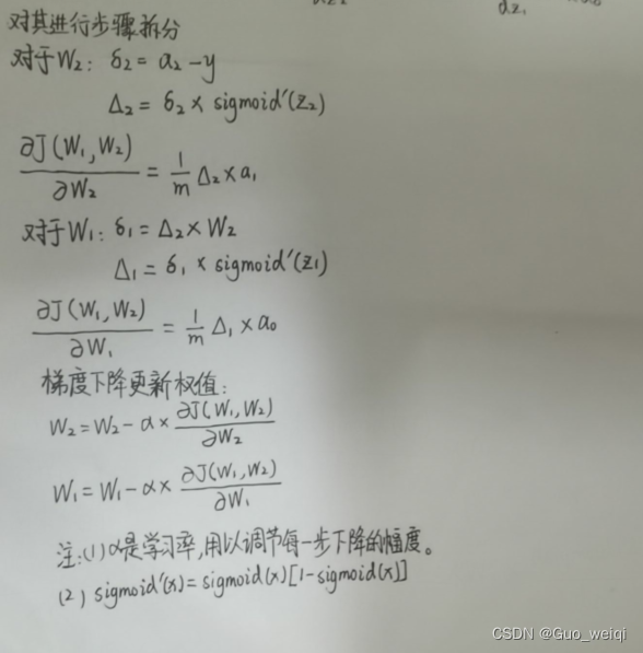
过程推导 - 了解BP原理
数值计算 - 手动计算，掌握细节
代码实现 - numpy手推 + pytorch自动
过程推导、数值计算，以下三种形式可任选其一：

 

 

直接在博客用编辑器写
在电子设备手写，截图
在纸上写，拍照发图
代码实现：

numpy: 

import numpy as np
 
w1, w2, w3, w4, w5, w6, w7, w8 = 0.2, -0.4, 0.5, 0.6, 0.1, -0.5, -0.3, 0.8
x1, x2 = 0.5, 0.3
y1, y2 = 0.23, -0.07
print("输入值 x0, x1:")
print(x1, x2)
print("输出值 y0, y1:")
print(y1, y2)
 
 
def sigmoid(z):
    a = 1 / (1 + np.exp(-z))
    return a
 
 
def forward_propagate(x1, x2, y1, y2, w1, w2, w3, w4, w5, w6, w7, w8):
    in_h1 = w1 * x1 + w3 * x2
    out_h1 = sigmoid(in_h1)
    in_h2 = w2 * x1 + w4 * x2
    out_h2 = sigmoid(in_h2)
 
    in_o1 = w5 * out_h1 + w7 * out_h2
    out_o1 = sigmoid(in_o1)
    in_o2 = w6 * out_h1 + w8 * out_h2
    out_o2 = sigmoid(in_o2)
 
    print("正向计算:预测值o1 ,o2为")
    print(round(out_o1, 5), round(out_o2, 5))
 
    error = (1 / 2) * (out_o1 - y1) ** 2 + (1 / 2) * (out_o2 - y2) ** 2
 
    print("损失函数(均方误差)：",round(error, 5))
 
    return out_o1, out_o2, out_h1, out_h2
 
 
def back_propagate(out_o1, out_o2, out_h1, out_h2):
    # 反向传播
    d_o1 = out_o1 - y1
    d_o2 = out_o2 - y2
 
    d_w5 = d_o1 * out_o1 * (1 - out_o1) * out_h1
    d_w7 = d_o1 * out_o1 * (1 - out_o1) * out_h2
    d_w6 = d_o2 * out_o2 * (1 - out_o2) * out_h1
    d_w8 = d_o2 * out_o2 * (1 - out_o2) * out_h2
 
    d_w1 = (d_o1 * out_h1 * (1 - out_h1) * w5 + d_o2 * out_o2 * (1 - out_o2) * w6) * out_h1 * (1 - out_h1) * x1
    d_w3 = (d_o1 * out_h1 * (1 - out_h1) * w5 + d_o2 * out_o2 * (1 - out_o2) * w6) * out_h1 * (1 - out_h1) * x2
    d_w2 = (d_o1 * out_h1 * (1 - out_h1) * w7 + d_o2 * out_o2 * (1 - out_o2) * w8) * out_h2 * (1 - out_h2) * x1
    d_w4 = (d_o1 * out_h1 * (1 - out_h1) * w7 + d_o2 * out_o2 * (1 - out_o2) * w8) * out_h2 * (1 - out_h2) * x2
 
    print("反向传播：误差传给每个权值", round(d_w1, 5), round(d_w2, 5), round(d_w3, 5), round(d_w4, 5), round(d_w5, 5), round(d_w6, 5),
          round(d_w7, 5), round(d_w8, 5))
 
    return d_w1, d_w2, d_w3, d_w4, d_w5, d_w6, d_w7, d_w8
 
 
def update_w(w1, w2, w3, w4, w5, w6, w7, w8):
    # 步长
    step = 1
    w1 = w1 - step * d_w1
    w2 = w2 - step * d_w2
    w3 = w3 - step * d_w3
    w4 = w4 - step * d_w4
    w5 = w5 - step * d_w5
    w6 = w6 - step * d_w6
    w7 = w7 - step * d_w7
    w8 = w8 - step * d_w8
    return w1, w2, w3, w4, w5, w6, w7, w8
 
 
if __name__ == "__main__":
 
    print("更新前的权值:",round(w1, 2), round(w2, 2), round(w3, 2), round(w4, 2), round(w5, 2), round(w6, 2), round(w7, 2),
          round(w8, 2))
 
    for i in range(1):
        print("第" + str(i+1) + "轮:")
        out_o1, out_o2, out_h1, out_h2 = forward_propagate(x1, x2, y1, y2, w1, w2, w3, w4, w5, w6, w7, w8)
        d_w1, d_w2, d_w3, d_w4, d_w5, d_w6, d_w7, d_w8 = back_propagate(out_o1, out_o2, out_h1, out_h2)
        w1, w2, w3, w4, w5, w6, w7, w8 = update_w(w1, w2, w3, w4, w5, w6, w7, w8)
 
    print("更新后的权值w:", round(w1, 2), round(w2, 2), round(w3, 2), round(w4, 2), round(w5, 2), round(w6, 2), round(w7, 2),
          round(w8, 2))

pytorch:

import torch

x1, x2 = torch.Tensor([0.5]), torch.Tensor([0.3])
y1, y2 = torch.Tensor([0.23]), torch.Tensor([-0.07])
print("=====输入值：x1, x2；真实输出值：y1, y2=====")
print(x1, x2, y1, y2)
w1, w2, w3, w4, w5, w6, w7, w8 = torch.Tensor([0.2]), torch.Tensor([-0.4]), torch.Tensor([0.5]), torch.Tensor(
    [0.6]), torch.Tensor([0.1]), torch.Tensor([-0.5]), torch.Tensor([-0.3]), torch.Tensor([0.8])  # 权重初始值
w1.requires_grad = True
w2.requires_grad = True
w3.requires_grad = True
w4.requires_grad = True
w5.requires_grad = True
w6.requires_grad = True
w7.requires_grad = True
w8.requires_grad = True


def sigmoid(z):
    a = 1 / (1 + torch.exp(-z))
    return a


def forward_propagate(x1, x2):
    in_h1 = w1 * x1 + w3 * x2
    out_h1 = sigmoid(in_h1)  # out_h1 = torch.sigmoid(in_h1)
    in_h2 = w2 * x1 + w4 * x2
    out_h2 = sigmoid(in_h2)  # out_h2 = torch.sigmoid(in_h2)

    in_o1 = w5 * out_h1 + w7 * out_h2
    out_o1 = sigmoid(in_o1)  # out_o1 = torch.sigmoid(in_o1)
    in_o2 = w6 * out_h1 + w8 * out_h2
    out_o2 = sigmoid(in_o2)  # out_o2 = torch.sigmoid(in_o2)

    print("正向计算：o1 ,o2")
    print(out_o1.data, out_o2.data)

    return out_o1, out_o2


def loss_fuction(x1, x2, y1, y2):  # 损失函数
    y1_pred, y2_pred = forward_propagate(x1, x2)  # 前向传播
    loss = (1 / 2) * (y1_pred - y1) ** 2 + (1 / 2) * (y2_pred - y2) ** 2  # 考虑 ： t.nn.MSELoss()
    print("损失函数（均方误差）：", loss.item())
    return loss


def update_w(w1, w2, w3, w4, w5, w6, w7, w8):
    # 步长
    step = 1
    w1.data = w1.data - step * w1.grad.data
    w2.data = w2.data - step * w2.grad.data
    w3.data = w3.data - step * w3.grad.data
    w4.data = w4.data - step * w4.grad.data
    w5.data = w5.data - step * w5.grad.data
    w6.data = w6.data - step * w6.grad.data
    w7.data = w7.data - step * w7.grad.data
    w8.data = w8.data - step * w8.grad.data
    w1.grad.data.zero_()  # 注意：将w中所有梯度清零
    w2.grad.data.zero_()
    w3.grad.data.zero_()
    w4.grad.data.zero_()
    w5.grad.data.zero_()
    w6.grad.data.zero_()
    w7.grad.data.zero_()
    w8.grad.data.zero_()
    return w1, w2, w3, w4, w5, w6, w7, w8


if __name__ == "__main__":

    print("=====更新前的权值=====")
    print(w1.data, w2.data, w3.data, w4.data, w5.data, w6.data, w7.data, w8.data)

    for i in range(1):
        print("=====第" + str(i) + "轮=====")
        L = loss_fuction(x1, x2, y1, y2)  # 前向传播，求 Loss，构建计算图
        L.backward()  # 自动求梯度，不需要人工编程实现。反向传播，求出计算图中所有梯度存入w中
        print("\tgrad W: ", round(w1.grad.item(), 2), round(w2.grad.item(), 2), round(w3.grad.item(), 2),
              round(w4.grad.item(), 2), round(w5.grad.item(), 2), round(w6.grad.item(), 2), round(w7.grad.item(), 2),
              round(w8.grad.item(), 2))
        w1, w2, w3, w4, w5, w6, w7, w8 = update_w(w1, w2, w3, w4, w5, w6, w7, w8)

    print("更新后的权值")
    print(w1.data, w2.data, w3.data, w4.data, w5.data, w6.data, w7.data, w8.data)

 

对比【numpy】和【pytorch】程序，总结并陈述。

两种方法的求解效果基本相同。
激活函数Sigmoid用PyTorch自带函数torch.sigmoid()，观察、总结并陈述。

使用Sigmoid函数和使用Pytorch自带函数torch.sigmoid()没较为明显的差距。
激活函数Sigmoid改变为Relu，观察、总结并陈述。

损失函数MSE用PyTorch自带函数 t.nn.MSELoss()替代，观察、总结并陈述。

def loss_fuction(x1, x2, y1, y2):  # 损失函数
    y1_pred, y2_pred = forward_propagate(x1, x2)  # 前向传播
    loss_func = torch.nn.MSELoss() # 创建损失函数
    y_pred = torch.cat((y1_pred, y2_pred), dim=0) # 将y1_pred, y2_pred合并成一个向量
    y = torch.cat((y1, y2), dim=0) # 将y1, y2合并成一个向量
    loss = loss_func(y_pred, y) # 计算损失
    print("损失函数（均方误差）：", loss.item())
    return loss

运行结果相同。
损失函数MSE改变为交叉熵，观察、总结并陈述。

def loss_fuction(x1, x2, y1, y2):
    y1_pred, y2_pred = forward_propagate(x1, x2)
    loss_func = torch.nn.CrossEntropyLoss() # 创建交叉熵损失函数
    y_pred = torch.stack([y1_pred, y2_pred], dim=1)
    y = torch.stack([y1, y2], dim=1)
    loss = loss_func(y_pred, y) # 计算
    print("损失函数（交叉熵损失）：", loss.item())
    return loss

改为交叉熵之后损失函数出现负数。
改变步长，训练次数，观察、总结并陈述。

步长越大，均方误差下降越快，收敛就越快，改变步数发现，随着步数的增大，均方误差下降速度也在逐渐降低，收敛速度下降。
权值w1-w8初始值换为随机数，对比“指定权值”的结果，观察、总结并陈述。

​w1, w2, w3, w4, w5, w6, w7, w8 = torch.randn(1), torch.randn(1), torch.randn(1), torch.randn(1), \
    torch.randn(1), torch.randn(1), torch.randn(1), torch.randn(1)

=====输入值：x1, x2；真实输出值：y1, y2=====
tensor([0.5000]) tensor([0.3000]) tensor([0.2300]) tensor([-0.0700])
=====更新前的权值=====
tensor([-0.3827]) tensor([1.1477]) tensor([0.3640]) tensor([0.4843]) tensor([-0.6357]) tensor([0.6936]) tensor([-0.2005]) tensor([-0.0979])
=====第0轮=====
正向计算：o1 ,o2
tensor([0.3918]) tensor([0.5663])
损失函数（均方误差）： 0.215525820851326
	grad W:  0.01 -0.0 0.01 -0.0 0.02 0.07 0.03 0.11
更新后的权值
tensor([-0.3931]) tensor([1.1503]) tensor([0.3577]) tensor([0.4858]) tensor([-0.6542]) tensor([0.6187]) tensor([-0.2265]) tensor([-0.2030])

权值w1-w8初始值换为0，观察、总结并陈述。

w1, w2, w3, w4, w5, w6, w7, w8 = torch.Tensor([0]), torch.Tensor([0]), torch.Tensor([0]), torch.Tensor(
    [0]), torch.Tensor([0]), torch.Tensor([0]), torch.Tensor([0]), torch.Tensor([0])

全面总结反向传播原理和编码实现，认真写心得体会。

BP算法是神经网络用于更新权值的算法，可以说是能让神经网络开始“学习”的核心，所以理解这个算法是非常重要的。本着实践是检验是否理解的唯一标准的原则，我借用了另一位博主的博客代码，稍微修改了一些地方，最后分析算法的结果。更加深刻理解了BP算法。