


遥感图像场景分类是指对遥感图像中场景语义内容标签的映射过程,对高分辨率遥感影像的信息提取及内容理解有着重要的意义。主要的场景分类方法可以分为三类:第一类是基于底层视觉特征的场景分类方法,第二类是基于中层视觉表示的场景分类方法,第三类是基于高层视觉信息的场景分类方法。其中基于高层视觉信息的场景分类方法通过训练卷积神经网络模型来自动提取图像的抽象语义特征,卷积神经网络展现出很强的图像场景特征描述能力,解决了底层、中层特征对场景语义信息描述不准确的问题,打开了大幅提升场景分类效果的大门。
为实现遥感图像的场景分类任务,我们自主设计一个卷积神经网络模型,并对分类结果进行评价,训练测试模型时选用的是21类场景分类遥感数据集UC Merced Land-Use,具体实现步骤如下。
- 下载遥感图像场景分类数据集UC Merced Land-Use →提取码:txeu。
- 配置基础环境:1) Windows10 + Anaconda3 + PyCharm 2019.3.3;
2) 安装CPU版本的TensorFlow;
3) 在PyCharm中配置好TensorFlow环境。 - 在PyCharm中新建场景分类项目
Scene-Classification并配置好TensorFlow环境,具体步骤参见使用卷积神经网络实现猫狗分类任务训练及测试过程中的1-2步。

- 新建好项目后,在训练模型之前需要对数据集进行处理。首先在下载的
UCMerced_LandUse文件夹中新建train、validation、test文件夹,并将Images文件夹下的所有文件复制到train文件夹中。

- 新建文件
get_filename.py用于获取数据集中各类别的名称,新建文件的具体步骤参见使用卷积神经网络实现猫狗分类任务训练及测试过程中的第3步。get_filename.py文件的代码如下所示。
import os

train_dir = 'E:/Remote Sensing/Scene-Classification/NWPU-RESISC45/train/'
for filename in os.listdir(train_dir):
    print(filename)
- 新建文件
create_file.py用于在validation、test文件夹中分别创建21个类别的子文件夹,代码如下所示。
import os

# UCMerced_LandUse
CLASS = ('agricultural', 'airplane', 'baseballdiamond', 'beach', 'buildings',
         'chaparral', 'denseresidential', 'forest', 'freeway', 'golfcourse', 'harbor',
         'intersection', 'mediumresidential', 'mobilehomepark', 'overpass', 'parkinglot',
         'river', 'runway', 'sparseresidential', 'storagetanks', 'tenniscourt')  # 此处的类别名称可由get_filename.py文件的运行结果得到
num = len(CLASS)
for i in range(num):
    validation_dir = 'E:/Remote Sensing/Data Set/UCMerced_LandUse/validation/'
    test_dir = 'E:/Remote Sensing/Data Set/UCMerced_LandUse/test/'
    # test_dir = 'E:/Remote Sensing/Scene-Classification/NWPU-RESISC45/test/'
    os.mkdir(os.path.join(validation_dir, CLASS[i]))
    os.mkdir(os.path.join(test_dir, CLASS[i]))
运行代码后的结果如下图所示。

- 新建文件
devide.py用于将数据集中的所有样本按比例划分为训练集、验证集和测试集,代码如下所示。
import os, random, shutil


def moveFile(fileDir, tarDir):
    pathDir = os.listdir(fileDir)  # 取图片的原始路径
    filenumber = len(pathDir)
    rate = 0.1  # 自定义抽取图片的比例,比方说100张抽10张,那就是0.1
    picknumber = int(filenumber * rate)  # 按照rate比例从文件夹中取一定数量图片
    sample = random.sample(pathDir, picknumber)  # 随机选取picknumber数量的样本图片
    print(sample)
    for name in sample:
        shutil.move(fileDir + '/' + name, tarDir + '/' + name)
    return


if __name__ == '__main__':
    train_dir = 'E:/Remote Sensing/Data Set/UCMerced_LandUse/train/'
    validation_dir = 'E:/Remote Sensing/Data Set/UCMerced_LandUse/validation'
    test_dir = 'E:/Remote Sensing/Data Set/UCMerced_LandUse/test/'
    # UCMerced_LandUse
    CLASS = ('agricultural', 'airplane', 'baseballdiamond', 'beach', 'buildings',
             'chaparral', 'denseresidential', 'forest', 'freeway', 'golfcourse', 'harbor',
             'intersection', 'mediumresidential', 'mobilehomepark', 'overpass', 'parkinglot',
             'river', 'runway', 'sparseresidential', 'storagetanks', 'tenniscourt')
    num = len(CLASS)
    for i in range(num):
        fileDir = os.path.join(train_dir, CLASS[i])
        tarDir1 = os.path.join(validation_dir, CLASS[i])
        moveFile(fileDir, tarDir1)
        tarDir2 = os.path.join(test_dir, CLASS[i])
        moveFile(fileDir, tarDir2)
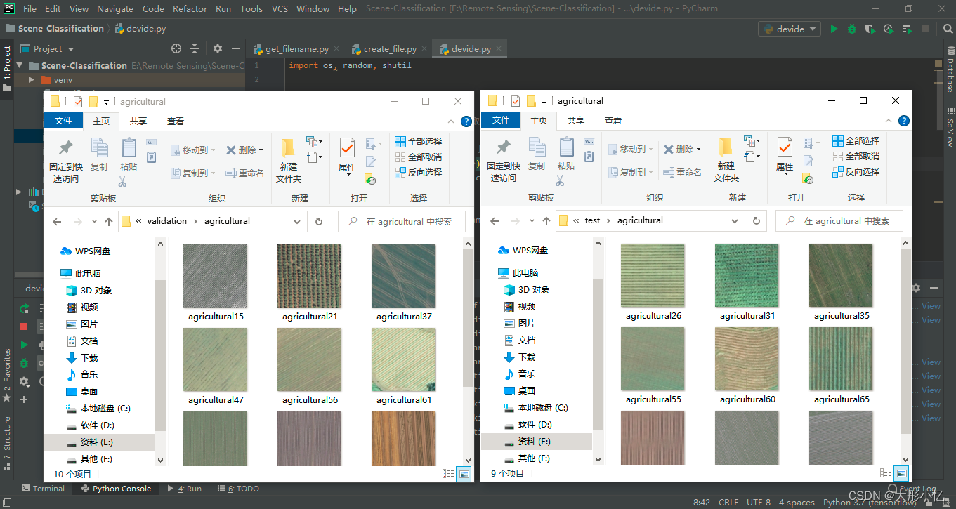
运行代码后的结果如下图所示。
- 新建文件
classification_DataEnhancement.py用于设计卷积神经网络模型并进行训练以实现场景分类,代码如下所示。
import os
import tensorflow as tf
from tensorflow.keras.optimizers import RMSprop
from tensorflow.keras.preprocessing.image import ImageDataGenerator
import matplotlib.pyplot as plt


base_dir = 'E:/Remote Sensing/Data Set/UCMerced_LandUse/'
# 指定每一种数据的位置
train_dir = os.path.join(base_dir, 'train')
validation_dir = os.path.join(base_dir, 'validation')

# UCMerced_LandUse
CLASS = ('agricultural', 'airplane', 'baseballdiamond', 'beach', 'buildings',
         'chaparral', 'denseresidential', 'forest', 'freeway', 'golfcourse', 'harbor',
         'intersection', 'mediumresidential', 'mobilehomepark', 'overpass', 'parkinglot',
         'river', 'runway', 'sparseresidential', 'storagetanks', 'tenniscourt')
num = len(CLASS)
for i in range(num):
    train_class_dir = os.path.join(train_dir, CLASS[i])
    validation_class_dir = os.path.join(validation_dir, CLASS[i])

# 设计模型
model = tf.keras.models.Sequential([
    # 我们的数据是150x150而且是三通道的,所以我们的输入应该设置为这样的格式。
    tf.keras.layers.Conv2D(32, (3, 3), activation='relu', input_shape=(256, 256, 3)),
    tf.keras.layers.MaxPooling2D(2, 2),
    tf.keras.layers.Conv2D(64, (3, 3), activation='relu'),
    tf.keras.layers.MaxPooling2D(3, 3),
    tf.keras.layers.Conv2D(128, (3, 3), activation='relu'),
    tf.keras.layers.MaxPooling2D(2, 2),
    tf.keras.layers.Conv2D(128, (3, 3), activation='relu'),
    tf.keras.layers.MaxPooling2D(2, 2),
    # tf.keras.layers.Dropout(0.5),
    # Flatten the results to feed into a DNN
    tf.keras.layers.Flatten(),
    # 512 neuron hidden layer
    tf.keras.layers.Dense(512, activation='relu'),
    tf.keras.layers.Dense(21, activation='softmax')  #'sigmoid'
])
model.summary()  # 打印模型相关信息

# 进行优化方法选择和一些超参数设置
# 因为只有两个分类。所以用2分类的交叉熵,使用RMSprop,学习率为0.001.优化指标为accuracy
model.compile(optimizer=RMSprop(lr=0.001),
              # loss='binary_crossentropy',
              loss='categorical_crossentropy',
              metrics=['acc'])

# 数据处理
train_datagen = ImageDataGenerator(
    rescale=1. / 255,
    rotation_range=40,
    width_shift_range=0.2,
    height_shift_range=0.2,
    shear_range=0.2,
    zoom_range=6.2,
    horizontal_flip=True, )

# Note that the validation data should not be augmented!(注意,不能增强验证数据)
test_datagen = ImageDataGenerator(rescale=1. / 255)
train_generator = train_datagen.flow_from_directory(
    # This is the target directory (目标目录)
    train_dir,
    # All images will be resized to 150x150(将所有图像的大小调整为150x150)
    target_size=(256, 256),
    batch_size=20,
    class_mode='categorical')  # 多分类

# 生成验证集带标签的数据
validation_generator = test_datagen.flow_from_directory(validation_dir,  # 验证图片的位置
                                                        batch_size=20,  # 每一个投入多少张图片训练
                                                        # class_mode='binary',  # 设置我们需要的标签类型
                                                        class_mode='categorical',  # 多分类
                                                        target_size=(256, 256))  # 将图片统一大小

# 进行训练
history = model.fit_generator(train_generator,                            validation_data=validation_generator,
                              steps_per_epoch=100,
                              epochs=200,
                              validation_steps=50,
                              verbose=2)
# pip install h5py
model.save('model_UCMerced_LandUse.h5')

# 得到精度和损失值
acc = history.history['acc']
val_acc = history.history['val_acc']
loss = history.history['loss']
val_loss = history.history['val_loss']
epochs = range(len(acc))  # 得到迭代次数
# 绘制精度曲线
plt.plot(epochs, acc)
plt.plot(epochs, val_acc)
plt.title('Training and validation accuracy')
plt.legend(('Training accuracy', 'validation accuracy'))
plt.figure()

# 绘制损失曲线
plt.plot(epochs, loss)
plt.plot(epochs, val_loss)
plt.legend(('Training loss', 'validation loss'))
plt.title('Training and validation loss')
plt.show()
运行代码后在根路径下得到最终模型model_UCMerced_LandUse.h5及精度曲线和损失曲线。
- 新建文件
predict.py用于对需要测试的图片进行类别预测,代码如下所示。
# 预测
from tensorflow.keras.models import load_model
import numpy as np
from tensorflow.keras.preprocessing import image

path = 'E:/Remote Sensing/Data Set/UCMerced_LandUse/test/forest/forest20.tif'
model = load_model('model_UCMerced_LandUse.h5')
img = image.load_img(path, target_size=(256, 256))
x = image.img_to_array(img) / 255.0
# 在第0维添加维度变为1x150x150x3,和我们模型的输入数据一样
x = np.expand_dims(x, axis=0)
# np.vstack:按垂直方向(行顺序)堆叠数组构成一个新的数组,我们一次只有一个数据所以不这样也可以
images = np.vstack([x])
# batch_size批量大小,程序会分批次地预测测试数据,这样比每次预测一个样本会快。因为我们也只有一个测试所以不用也可以
classes1 = model.predict(images, batch_size=10)
print(classes1)
classes = model.predict_classes(images)
ind = classes[0]
print(ind)
# UCMerced_LandUse
CLASS = ('agricultural', 'airplane', 'baseballdiamond', 'beach', 'buildings',
         'chaparral', 'denseresidential', 'forest', 'freeway', 'golfcourse', 'harbor',
         'intersection', 'mediumresidential', 'mobilehomepark', 'overpass', 'parkinglot',
         'river', 'runway', 'sparseresidential', 'storagetanks', 'tenniscourt')
print("It is ", CLASS[ind])
运行代码后的结果如下图所示。

- 新建文件
visual.py用于可视化每个卷积层的特征图,代码如下所示。
import numpy as np
import matplotlib.pyplot as plt
from tensorflow.keras.preprocessing.image import img_to_array, load_img
import tensorflow as tf
from tensorflow.keras.models import load_model

np.seterr(divide='ignore', invalid='ignore')
model = load_model('model_UCMerced_LandUse.h5')
# 让我们定义一个新模型,该模型将图像作为输入,并输出先前模型中所有层的中间表示。
successive_outputs = [layer.output for layer in model.layers[1:]]
# 进行可视化模型搭建,设置输入和输出
visualization_model = tf.keras.models.Model(inputs=model.input, outputs=successive_outputs)
# 选取一张随机的图片
img_path = 'E:/Remote Sensing/Data Set/UCMerced_LandUse/test//beach/beach15.tif'
img = load_img(img_path, target_size=(256, 256))  # 以指定大小读取图片
x = img_to_array(img)  # 变成array
x = x.reshape((1,) + x.shape)  # 变成 (1, 150, 150, 3)
# 统一范围到0到1
x /= 255
# 运行我们的模型,得到我们要画的图。
successive_feature_maps = visualization_model.predict(x)
# 选取每一层的名字
layer_names = [layer.name for layer in model.layers]
# 开始画图
for layer_name, feature_map in zip(layer_names, successive_feature_maps):
    if len(feature_map.shape) == 4:
        # 只绘制卷积层,池化层,不画全连接层。
        n_features = feature_map.shape[-1]  # 最后一维的大小,也就是通道数,也是我们提取的特征数
        # feature_map的形状为 (1, size, size, n_features)
        size = feature_map.shape[1]
        # 我们将在此矩阵中平铺图像
        display_grid = np.zeros((size, size * n_features))
        for i in range(n_features):
            # 后期处理我们的特征,使其看起来更美观。
            x = feature_map[0, :, :, i]
            x -= x.mean()
            x /= x.std()
            x *= 64
            x += 128
            x = np.clip(x, 0, 255).astype('uint8')
            # 我们把图片平铺到这个大矩阵中
            display_grid[:, i * size: (i + 1) * size] = x
        # 绘制这个矩阵
        scale = 20. / n_features
        plt.figure(figsize=(scale * n_features, scale))  # 设置图片大小
        plt.title(layer_name)  # 设置题目
        plt.grid(False)  # 不绘制网格线
        # aspect='auto'自动控制轴的长宽比。 这方面对于图像特别相关,因为它可能会扭曲图像,即像素不会是正方形的。
        # cmap='viridis'设置图像的颜色变化
        plt.imshow(display_grid, aspect='auto', cmap='viridis')
        plt.show()
运行代码后可依次得到每一个卷积层的特征图,结果如下图所示。


 7065
7065


 被折叠的 条评论
为什么被折叠?
被折叠的 条评论
为什么被折叠?
 到【灌水乐园】发言


