


数学启发式算法 | 手把手教你 Python+Gurobi 实现可行性泵 (Feasibility Pump)算法
- 数学规划与线性规划
- 混合整数规划(Mixed Integer Porgramming, MIP)及其复杂度
- 获得MIP可行解的经典数学启发式算法:可行性泵算法(Feasibility Pump)
- Python+Gurobi实现Feasibility Pump:简单案例
- Python+Gurobi实现Feasibility Pump:VRPTW (Solomon VRP benchmark )
- 数值实验1:C101: 50 customers + 5 vehicles
- 不使用Feasibility Pump: Branch and bound + pseudo cost branching
- 使用Feasibility Pump: Branch and bound + pseudo cost branching + FP
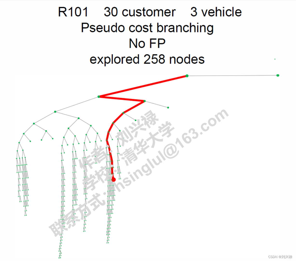
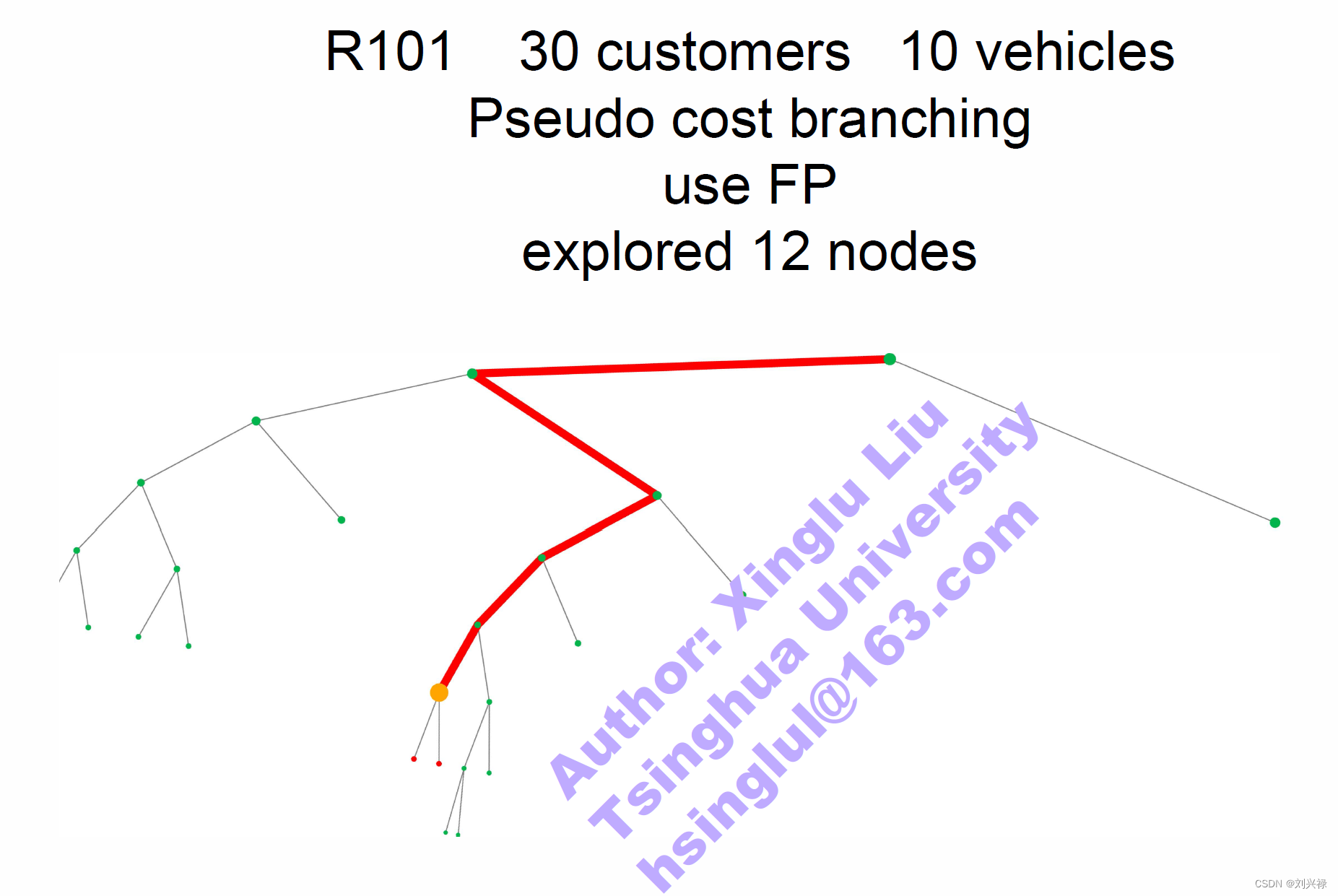
- 数值实验2:R101: 30 customers + 3 vehicles
- 不使用Feasibility Pump: Branch and bound + pseudo cost branching
- 使用Feasibility Pump: Branch and bound + pseudo cost branching + FP
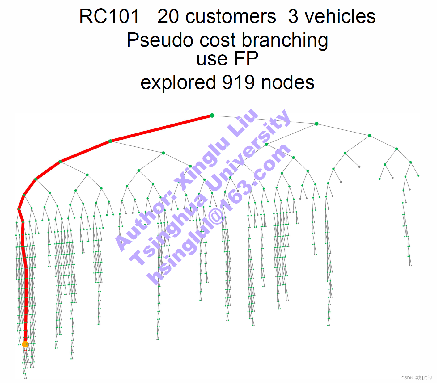
- 数值实验3:RC101: 20 customers + 3 vehicles
- 不使用Feasibility Pump: Branch and bound + pseudo cost branching
- 使用Feasibility Pump: Branch and bound + pseudo cost branching + FP
- 小结
- 参考文献
作者:刘兴禄,清华大学,清华大学深圳国际研究生院,清华-伯克利深圳学院,博士在读,邮箱:hsinglul@163.com
作者:陈懋宁,清华大学,清华大学深圳国际研究生院,硕士在读,邮箱:catme1008@163.com
欢迎关注我们的微信公众号 运小筹

数学规划与线性规划
数学规划(Mathematical Programming)是一种考虑约束和目标函数的约束优化技术。我们熟知的线性规划(Linear Programming)就是一类最简单的数学规划,其一般形式如下:
max
c
T
x
s
.
t
.
A
x
⩽
b
,
x
⩾
0.
x
∈
R
n
.
\begin{aligned} \max \quad &\mathbf{c}^T \mathbf{x} \\ s.t. \quad& \mathbf{A}\mathbf{x} \leqslant \mathbf{b}, \\ &\mathbf{x} \geqslant \mathbf{0}. \\ &\mathbf{x} \in \mathbb{R}^n. \end{aligned}
maxs.t.cTxAx⩽b,x⩾0.x∈Rn.
其中,
c
∈
R
n
×
1
\mathbf{c} \in \mathbb{R}^{n\times 1}
c∈Rn×1,为列向量(所以
c
T
\mathbf{c}^T
cT为行向量),
x
∈
R
n
×
1
\mathbf{x} \in \mathbb{R}^{n\times 1}
x∈Rn×1,为列向量,
A
∈
R
m
×
n
\mathbf{A} \in \mathbb{R}^{m\times n}
A∈Rm×n, 为约束系数矩阵,
b
∈
R
m
×
1
\mathbf{b} \in \mathbb{R}^{m\times 1}
b∈Rm×1,为列向量(Right Hand Side)。一个简单的线性规划的例子如下:
max
x
1
+
x
2
s
.
t
.
x
1
+
2
x
2
⩽
6
,
x
1
+
x
2
⩽
5
,
x
1
,
x
2
⩾
0.
\begin{aligned} \max \quad & x_1 + x_2 \\ s.t. \quad& x_1 + 2x_2 \leqslant 6, \\ & x_1 + x_2 \leqslant 5, \\ &x_1, x_2 \geqslant 0. \end{aligned}
maxs.t.x1+x2x1+2x2⩽6,x1+x2⩽5,x1,x2⩾0.
线性规划已经被证明是可以用内点法(Interior method or barrier method)在多项式时间内精确求解的,见文献1。不过在具体实践中,单纯形法(Simplex method)也非常快,不过Simplex method是非多项式时间算法。
关于线性规划的更加详细的即介绍,再次不做过多介绍,之后有机会再详细阐述。我们快速聚焦到今天的主题:混合整数规划。
混合整数规划(Mixed Integer Porgramming, MIP)及其复杂度
若线性规划中的所有决策变量均要求取值为整数时,模型变化为整数规划(Integer Porgramming, IP),也叫纯整数规划(Pure Integer Porgramming)。整数规划的一般形式为
max
c
T
x
s
.
t
.
A
x
⩽
b
,
x
∈
Z
n
.
\begin{aligned} \max \quad &\mathbf{c}^T \mathbf{x} \\ s.t. \quad& \mathbf{A}\mathbf{x} \leqslant \mathbf{b}, \\ &\mathbf{x} \in \mathbb{Z}^n. \end{aligned}
maxs.t.cTxAx⩽b,x∈Zn.
如果考虑决策变量汇总有一部分为整数变量,则该模型为混合整数规划(Mixed Integer Porgramming, MIP)。混合整数规划的一般形式如下:
max
c
T
x
+
d
T
y
s
.
t
.
A
x
+
B
y
⩽
b
,
x
∈
Z
n
,
y
∈
R
m
.
\begin{aligned} \max \quad &\mathbf{c}^T \mathbf{x} + \mathbf{d}^T \mathbf{y} \\ s.t. \quad& \mathbf{A}\mathbf{x} + \mathbf{B}\mathbf{y} \leqslant \mathbf{b}, \\ &\mathbf{x} \in \mathbb{Z}^n, \mathbf{y} \in \mathbb{R}^m. \end{aligned}
maxs.t.cTx+dTyAx+By⩽b,x∈Zn,y∈Rm.
其中,
c
∈
R
n
×
1
\mathbf{c} \in \mathbb{R}^{n\times 1}
c∈Rn×1,为列向量(所以
c
T
\mathbf{c}^T
cT为行向量),
d
∈
R
m
×
1
\mathbf{d} \in \mathbb{R}^{m\times 1}
d∈Rm×1,为列向量(所以
d
T
\mathbf{d}^T
dT为行向量),
x
∈
R
(
n
+
m
)
×
1
\mathbf{x} \in \mathbb{R}^{(n+m)\times 1}
x∈R(n+m)×1,为列向量,
A
∈
R
k
×
n
\mathbf{A} \in \mathbb{R}^{k\times n}
A∈Rk×n, 为约束系数矩阵,
B
∈
R
k
×
m
\mathbf{B} \in \mathbb{R}^{k\times m}
B∈Rk×m, 为约束系数矩阵,
b
∈
R
k
×
1
\mathbf{b} \in \mathbb{R}^{k\times 1}
b∈Rk×1,为列向量(Right Hand Side)。
注意到,混合整数规划如果不做特殊说明,指的都是混合整数线性规划(Mixed Integer Linear Porgramming, MILP)。一个简单的MIP的例子如下(也就是我们代码中采用的例子):
max
x
1
+
x
2
+
y
1
+
y
2
s
.
t
.
x
1
+
y
2
⩽
5
,
x
1
+
x
2
+
y
1
⩽
5.9
,
x
1
+
x
2
+
y
2
⩽
7.2
,
y
1
+
y
2
⩽
7.3
,
x
1
,
x
2
,
y
1
,
y
2
⩾
0
,
x
1
,
x
2
∈
N
.
\begin{aligned} \max \quad & x_1 + x_2 + y_1 + y_2 \\ s.t. \quad& x_1 + y_2 \leqslant 5, \\ & x_1 + x_2 + y_1 \leqslant 5.9, \\ & x_1 + x_2 + y_2 \leqslant 7.2, \\ & y_1 + y_2 \leqslant 7.3, \\ &x_1, x_2, y_1, y_2 \geqslant 0, \\ &x_1, x_2 \in \mathbb{N}. \end{aligned}
maxs.t.x1+x2+y1+y2x1+y2⩽5,x1+x2+y1⩽5.9,x1+x2+y2⩽7.2,y1+y2⩽7.3,x1,x2,y1,y2⩾0,x1,x2∈N.
混合整数规划已经被证明是NP-hard。以及,获得一个一般MIP模型的可行解,也是NP-hard。
获得MIP可行解的经典数学启发式算法:可行性泵算法(Feasibility Pump)
获得MIP可行解的复杂度
对于一个已知具体问题的MIP模型,例如车辆路径规划问题(Vehicle Routing Problem, VRP)、背包问题、设施选址问题等,我们可以根据问题的特性,使用一些启发式算法或者元启发式算法,快速获得可行解。例如,对于VRP问题,我们不用求解VRP的MIP模型,就可以直接使用插入算法(Insertion Algorithm)、节约算法(Saving Algorithm)、变邻域搜索算法(Variable Neighborhood Serach)、大规模自适应变邻域搜索算法(Adaptive Large Neighborhood Serach, ALNS)、遗传算法(Genetic Algorithm, GA)等方法,获得VRP的可行解。这些获得可行解的算法,一般都是多项式时间的。
但是对于一个一般的MIP模型,如果我们仅仅知道其决策变量和约束,却不知道它对应的具体问题是什么,则我们无法使用上述的启发式或者元启发式算法直接根据问题特性在多项式时间内保证得到可行解。此时,获得该一般MIP的可行解已经被证明是NP-hard。即:获得一个general MIP的可行解是NP-hard。
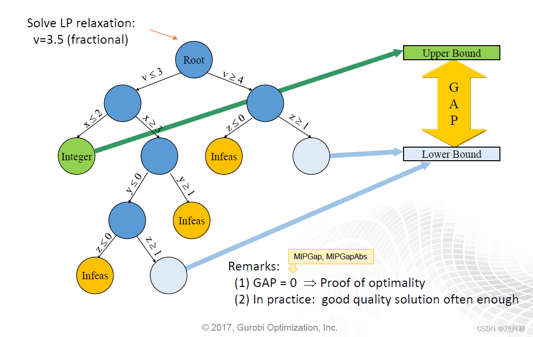
精确求解general的MIP,目前为止最快的算法为branch and cut框架。对于一个最大化问题(Maximization),其上界可以通过MIP的LP relaxation加cutting plane来获得,但是其下界的更新方式就只有一种:即获得更好的可行解。如下图所示(来自参考文献2)。
如何快速获得MIP的可行解呢?目前已有的方法主要有以下两大类:
- 基于LP的启发式
- 不基于LP的启发式。
具体的介绍,可以参考【运小筹】公众号的往期推文:【强大的数学启发式】
数学启发式算法:可行性泵算法(Feasibility Pump)
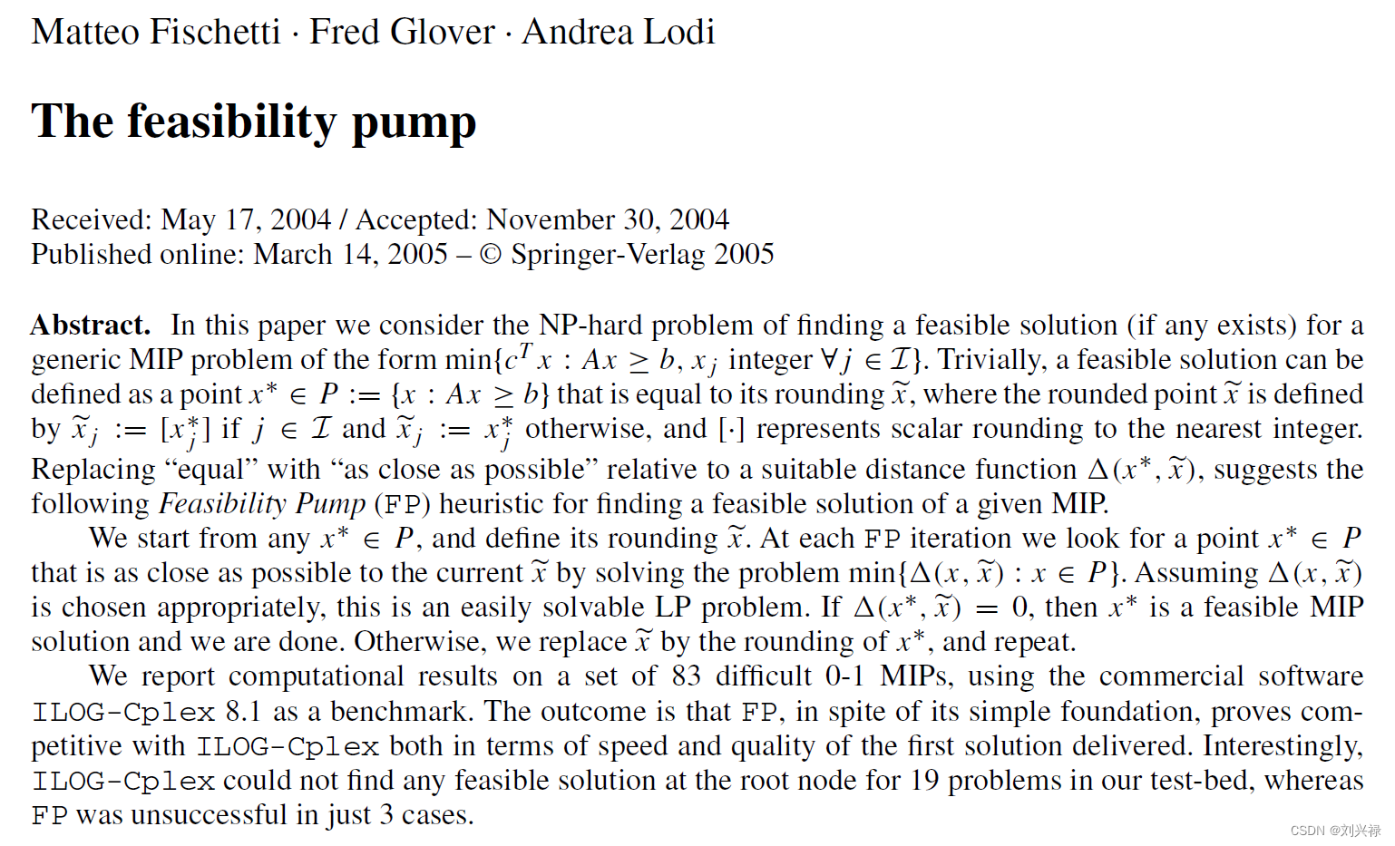
本文主要介绍一种非常经典的获得MIP可行解的算法:可行性泵算法(Feasibility Pump)。该算法于2005年由Matteo Fischetti、Fred Glover、Andrea Lodi提出,并发表在数学规划顶级期刊《Mathematical Programming》上,参考文献如下:
Fischetti M, Glover F, Lodi A. The feasibility pump[J]. Mathematical Programming, 2005, 104(1): 91-104.
值得一提的是,本推文的作者之一(刘兴禄)还有幸现场听过Fred Glover的讲座。Fred Glover在运筹学领域贡献巨大,著名的Tabu Search就是他提出的。为了表示对大佬的崇拜,这里我们贴上大佬的Google Scholar主页。

首先,我们来贴上这篇原始论文的摘要和Fesaibility Pump算法的伪代码:
详解Feasibility Pump
我们考虑下面的MIP
min c T x s.t. A x ⩾ b x j integer , ∀ j ∈ I \begin{aligned} \min \quad & \mathbf{c}^T \mathbf{x} \\ \text{s.t.} \quad & \mathbf{A}\mathbf{x} \geqslant \mathbf{b} \\ & x_j \text{ integer}, \forall j \in \mathcal{I} \end{aligned} mins.t.cTxAx⩾bxj integer,∀j∈I
用
x
∗
x^{*}
x∗表示上述MIP的线性松弛问题的最优解,即
x
∗
∈
P
=
{
x
∣
A
x
⩾
b
}
\begin{aligned} x^{*} \in P = \{ \mathbf{x}| \mathbf{A}\mathbf{x} \geqslant \mathbf{b} \} \end{aligned}
x∗∈P={x∣Ax⩾b}
Feasibility Pump要干的事儿,就是根据一个MIP的LP relaxation的小数解,通过构造新的目标函数,迭代获得一个整数可行解。下面我们来具体解释Feasibility Pump。
首先,我们定义:线性规划最优解的圆整解为 x ~ \tilde{x} x~。圆整解 x ~ \tilde{x} x~就是将LP relaxation的解 x ∗ x^{*} x∗通过四舍五入,圆整为整数(仅对整数决策变量进行圆整)。具体来讲:
-
如果这个变量是整数类型,即 j ∈ I j \in \mathcal{I} j∈I,则令
x ~ j = [ x j ∗ ] \begin{aligned} \tilde{x}_j = [x_j^{*}] \end{aligned} x~j=[xj∗]
其中 [ ⋅ ] [\cdot] [⋅]指的是圆整到距离他最近的整数。 -
如果该变量是连续变量,则令
x ~ j = x j ∗ \begin{aligned} \tilde{x}_j = x_j^{*} \end{aligned} x~j=xj∗
Feasibility Pump的思想就是,我们从一个 x j ∗ x_j^{*} xj∗开始,计算其对应的圆整解 x ~ \tilde{x} x~。然后我们通过更改目标函数,去尝试寻找与圆整解 x ~ \tilde{x} x~距离可能接近的LP relaxation解 x j ∗ x_j^{*} xj∗,直到找到一个距离为0的解,则说明找到了一个原问题的整数可行解。
怎么让下一个
x
j
∗
x_j^{*}
xj∗和其圆整解
x
~
\tilde{x}
x~尽可能接近呢?一个很直观的办法就是:定义一个圆整解
x
~
\tilde{x}
x~和LP relaxation解
x
j
∗
x_j^{*}
xj∗之间的距离函数,并让该距离尽可能小。假设二者的距离函数可以用
Δ
(
x
∗
,
x
~
)
\Delta (x^{*}, \tilde{x})
Δ(x∗,x~)表示,则我们要做的事情,就变成解如下的新的线性规划问题:
min
Δ
(
x
∗
,
x
~
)
s.t.
x
∈
P
\begin{aligned} \min \quad & \Delta (x^{*}, \tilde{x}) \\ \text{s.t.} \quad & x \in P \end{aligned}
mins.t.Δ(x∗,x~)x∈P
如果我们得到 Δ ( x ∗ , x ~ ) = 0 \Delta (x^{*}, \tilde{x}) =0 Δ(x∗,x~)=0,则我们就是得到了一个整数可行解 x ∗ x^{*} x∗。
但是,如何选取合适的 Δ ( x ∗ , x ~ ) \Delta (x^{*}, \tilde{x}) Δ(x∗,x~)呢?这个问题很关键。
文献3提出的办法是:使用 L 1 L_1 L1 norm,即设置 Δ ( x ∗ , x ~ ) \Delta (x^{*}, \tilde{x}) Δ(x∗,x~)的形式如下:
Δ ( x ∗ , x ~ ) = ∑ j ∈ J ∣ x j − x ~ j ∣ \begin{aligned} \Delta (x^{*}, \tilde{x})=\sum_{j \in \mathcal{J}}{|x_j-\widetilde {x}_j|} \end{aligned} Δ(x∗,x~)=j∈J∑∣xj−x j∣
注意,这一距离的计算仅包含整数变量 x j , ∀ j ∈ J x_j, \forall j \in \mathcal{J} xj,∀j∈J,不包含连续变量 x j , ∀ j ∉ J x_j, \forall j \notin \mathcal{J} xj,∀j∈/J. 进一步地,通过引入辅助变量 x i + , x i − x_i^+,x_i^- xi+,xi−,我们将上述模型进行线性化,对于整数变量 x j , ∀ j ∈ J x_j, \forall j \in \mathcal{J} xj,∀j∈J,有取值范围: l i ⩽ x i ⩽ u i , ∀ j ∈ J l_i \leqslant x_i \leqslant u_i,\forall j \in \mathcal{J} li⩽xi⩽ui,∀j∈J可以得到如下的等式:
Δ = ∑ j ∈ J , x ~ j = l j ( x j − l j ) + ∑ j ∈ J , x ~ j = u j ( u j − x j ) + ∑ j ∈ J , l j < x ~ j < u j ( x j + + x j − ) \begin{aligned} \Delta =\sum_{j \in \mathcal{J},\widetilde {x}_j=l_j}(x_j-l_j)+\sum_{j \in \mathcal{J},\widetilde {x}_j=u_j}(u_j-x_j)+\sum_{j \in \mathcal{J}, l_j < \widetilde {x}_j < u_j}(x_j^+ + x_j^-) \end{aligned} Δ=j∈J,x j=lj∑(xj−lj)+j∈J,x j=uj∑(uj−xj)+j∈J,lj<x j<uj∑(xj++xj−)
同时,增加约束:
x j = x ~ j + x j + − x j − , x j + ⩾ 0 , x j − ⩾ 0 , ∀ j ∈ J : l j < x ~ j < u j . \begin{aligned} x_j=\widetilde {x}_j+x_j^+ - x_j^- , x_j^+ \geqslant 0,x_j^- \geqslant 0, \quad \forall j \in \mathcal{J}:l_j < \widetilde {x}_j < u_j. \end{aligned} xj=x j+xj+−xj−,xj+⩾0,xj−⩾0,∀j∈J:lj<x j<uj.
这一约束中,将变量 x x x拆分为如下三个部分,第一部分 x ~ j \widetilde {x}_j x j是整数分量的值, x j + x_j^+ xj+ 和 x j − x_j^- xj−分别表示当 x j > x ~ j x_j>\widetilde {x}_j xj>x j和 x j < x ~ j x_j<\widetilde {x}_j xj<x j时解中分量 x j x_j xj与整数点对应分量 x ~ j \widetilde {x}_j x j的非负差值。综上,可以得到Feasibility Pump算法的线性规划模型(FP-LP),其目标函数为最小化距离 Δ ( x ∗ , x ~ ) \Delta (x^{*}, \tilde{x}) Δ(x∗,x~):
min ∑ j ∈ J , x ~ j = l j ( x j − l j ) + ∑ j ∈ J , x ~ j = u j ( u j − x j ) + ∑ j ∈ J , l j < x ~ j < u j ( x j + + x j − ) s.t. l b ⩽ x ⩽ u b , A x ⩾ b , x j = x ~ j + x j + − x j − , ∀ j ∈ J : l j < x ~ j < u j , x j + , x j − ⩾ 0 , ∀ j ∈ J : l j < x ~ j < u j . \begin{aligned} \min \quad &\sum_{j \in \mathcal{J},\widetilde {x}_j=l_j}(x_j-l_j)+\sum_{j \in \mathcal{J},\widetilde {x}_j=u_j}(u_j-x_j)+\sum_{j \in \mathcal{J},l_j < \widetilde {x}_j < u_j}(x_j^+ + x_j^-) \\ \text{s.t.} \quad & \mathbf{lb} \leqslant\mathbf{x} \leqslant \mathbf{ub}, \\ & \mathbf{Ax} \geqslant\mathbf{b}, \\ &x_j=\tilde {x}_j+x_j^+ - x_j^-, \quad \forall j \in \mathcal{J}:l_j < \widetilde {x}_j < u_j, \\ &x_j^+, x_j^- \geqslant 0, \,\,\quad \quad\quad\quad\forall j \in \mathcal{J}:l_j < \widetilde {x}_j < u_j. \end{aligned} mins.t.j∈J,x j=lj∑(xj−lj)+j∈J,x j=uj∑(uj−xj)+j∈J,lj<x j<uj∑(xj++xj−)lb⩽x⩽ub,Ax⩾b,xj=x~j+xj+−xj−,∀j∈J:lj<x j<uj,xj+,xj−⩾0,∀j∈J:lj<x j<uj.
注意,其中 x ~ j \tilde {x}_j x~j是上一次迭代中由上一次获得的 x j ∗ x_j^{*} xj∗通过圆整得到的圆整解 x ~ \tilde{x} x~,在该模型中 x ~ \tilde{x} x~为一个已知的参数。
显然,对于LP问题的解 x ∗ x^* x∗而言,当距离 Δ ( x ∗ , x ~ ) = 0 \Delta (x^{*}, \tilde{x})=0 Δ(x∗,x~)=0时,该解为整数解,而越小的距离,则代表当前解与整数解越接近。Feasibility Pump算法的思想是,将解的性质分为两类,可行性(Feasibility)与整数性(Integrality)。整数性很容易通过取整取得,而可行性则通过求解松弛问题(LP)取得。满足整数的点,不一定满足可行性,而满足可行性的点,不一定满足整性。从几何意义上见,可行解 x ∗ x^* x∗是多面体 P P P内部的点,而由取整得到的整数解 ( x ~ ) (\widetilde x) (x ) 则可能位于多面体内,也可能位于多面体外。Feasibility Pump算法将每此迭代成为‘泵周期(Pumping cycle)’,在每个周期内,多面体 P P P内部与上一整数解最近的点(可行解),通过对这一可行解进行圆整,实现了将可行性(Feasibility)泵入(Pumping)整数性的过程,并最终得到MIP的可行解。在几何上,Pumping过程会形成两条轨迹:一条是整数解 ( x ~ ) (\widetilde x) (x )的轨迹,另一条是LP relaxation可行解 ( x ∗ ) (x^*) (x∗)的轨迹,两条轨迹最终会交会的点即为MIP的可行解 ( x ~ ∗ ) (\widetilde x^*) (x ∗). 在Feasibility Pump中,采取线性的距离定义可以理解为是在一定程度上保证问题的线性。
通过梳理,我们自己整理了一下Feasibility Pump算法的流程,具体如下:
1.初始化算法,设置迭代次数为0
2.求解原问题的线性松弛问题(LP),如果此时原问题的解已经为整数,返回。
3.将LP的解进行圆整,得到整数解
4.当迭代次数小于规定的上限时,执行:
5.    迭代次数+1
6.    将整数解带入FP-LP中,并求解
7.    如果此时的可行解为整数,返回
8.    如果存在圆整后的可行解分量不与上次的整数解一致
9.       将圆整后的可行解作为整数解
10.   否则,遇到了驻点
11.       随机抽取一定的整数变量,反转(调换圆整方向,由四舍五入变为四入五舍)以增加距离,
Feasibility Pump迭代过程中的一些细节
我们还是把原文的伪代码贴过来:
这里需要注意,第9行的扰动操作。对于一个0-1整数规划,Feasibility Pump在每一次迭代过程中需要求解的问题是
min
Δ
(
x
∗
,
x
~
)
=
∑
j
∈
I
:
x
~
=
0
x
j
+
∑
j
∈
I
:
x
~
=
1
(
1
−
x
j
)
s.t.
x
∈
P
.
\begin{aligned} \min \quad & \Delta (x^{*}, \tilde{x}) = \sum_{j\in \mathcal I: \tilde{x}=0} x_j + \sum_{j\in \mathcal I: \tilde{x}=1} (1 - x_j) \\ \text{s.t.} \quad & x \in P. \end{aligned}
mins.t.Δ(x∗,x~)=j∈I:x~=0∑xj+j∈I:x~=1∑(1−xj)x∈P.
在迭代过程中, 上述模型会出现目标函数不再更新的情况,也就是上文中提到的,遇到了驻点。
比如下面的迭代过程:
FP_iter		FP_Obj			Last_Obj
1			8.981			0
2			2.445			8.981
3			1.890			2.445
4			1.890			1.890
5			1.890			1.890
可以看到,从第3步开始,目标函数不再变化。如果不做干涉,程序将会进入死循环。为了跳出死循环,我们需要对已经设置好的圆整解
x
~
=
[
x
∗
]
\tilde{x} = [x^*]
x~=[x∗]进行变化。我们首先对所有的
x
j
,
∀
j
∈
I
x_j, \forall j \in \mathcal{I}
xj,∀j∈I计算:
∣
x
j
∗
−
[
x
∗
]
∣
\begin{aligned} |x_j^{*} - [x^*] | \end{aligned}
∣xj∗−[x∗]∣
比如计算出来是
x[1] = 0.1
x[2] = 0.24
x[3] = 0.02
然后我们对其排序,排序之后,我们需要选择其中的一部分,将其 x ~ \tilde{x} x~进行变化。
x[2] = 0.24
x[1] = 0.1
x[3] = 0.02
比如,选择 ∣ x j ∗ − [ x ∗ ] ∣ |x_j^{*} - [x^*] | ∣xj∗−[x∗]∣最高的 x 2 x_2 x2,本来对应的 x ~ 2 = [ x 2 ∗ ] = [ 0.2 ] = 0 \tilde{x}_2 =[x_2^*] = [0.2] = 0 x~2=[x2∗]=[0.2]=0, 我们将其变化为 x ~ 2 = 1 \tilde{x}_2=1 x~2=1。
但是,要选择多少个
[
x
∗
]
[x^*]
[x∗]进行变化呢?这里,伪代码第9行说,我们可以给定一个需要变动的变量数的个数
T
T
T,然后我们随机在区间
[
T
2
,
3
T
2
]
\begin{aligned} [ \frac{T}{2}, \frac{3T}{2}] \end{aligned}
[2T,23T]
之间随机生成一个数,比如
random number
=
15
\text{random number} = 15
random number=15,也就是我们要将
∣
x
j
∗
−
[
x
∗
]
∣
|x_j^{*} - [x^*] |
∣xj∗−[x∗]∣排名前15的决策变量的圆整后的值进行变化,或者进行随机翻牌。
Python+Gurobi实现Feasibility Pump:简单案例
我们考虑如下的MIP。
max
x
1
+
x
2
+
y
1
+
y
2
s
.
t
.
x
1
+
y
2
⩽
5
,
x
1
+
x
2
+
y
1
⩽
5.9
,
x
1
+
x
2
+
y
2
⩽
7.2
,
y
1
+
y
2
⩽
7.3
,
x
1
,
x
2
,
y
1
,
y
2
⩾
0
,
x
1
,
x
2
∈
N
.
\begin{aligned} \max \quad & x_1 + x_2 + y_1 + y_2 \\ s.t. \quad& x_1 + y_2 \leqslant 5, \\ & x_1 + x_2 + y_1 \leqslant 5.9, \\ & x_1 + x_2 + y_2 \leqslant 7.2, \\ & y_1 + y_2 \leqslant 7.3, \\ &x_1, x_2, y_1, y_2 \geqslant 0, \\ &x_1, x_2 \in \mathbb{N}. \end{aligned}
maxs.t.x1+x2+y1+y2x1+y2⩽5,x1+x2+y1⩽5.9,x1+x2+y2⩽7.2,y1+y2⩽7.3,x1,x2,y1,y2⩾0,x1,x2∈N.
这里,我们使用Python调用Gurobi实现Feasibility Pump。
from gurobipy import *
import random
import math

class feasibility_pump():

    def __init__(self):
        # initialize
        self.MP = Model()
        self.iter = 0
        self.MAX_ITER = 30

    def load_problem(self):
        # add model
        mip = Model()
        # add constraints
        x1 = mip.addVar(0, GRB.INFINITY, vtype=GRB.CONTINUOUS, name='x1')
        x2 = mip.addVar(0, GRB.INFINITY, vtype=GRB.CONTINUOUS, name='x2')
        y1 = mip.addVar(0, GRB.INFINITY, vtype=GRB.CONTINUOUS, name='y1')
        y2 = mip.addVar(0, GRB.INFINITY, vtype=GRB.CONTINUOUS, name='y2')
        # add objective
        obj = LinExpr(0)
        obj.add(x1 + x2 + y1 + y2)
        mip.setObjective(obj, GRB.MAXIMIZE)
        # add constraints
        mip.addConstr(x1 + y2 <= 5, name='constr_1')
        mip.addConstr(x1 + x2 + y1 <= 5.9, name='constr_2')
        mip.addConstr(x1 + x2 + y2 <= 7.2, name='constr_3')
        mip.addConstr(y1 + y2 <= 7.3, name='constr_4')
        # load model
        mip.update()
        self.MP = mip

    def calc_distance(self, xs, x_integers):
        # calculate the distance
        s = 0
        for i in range(len(xs)):
            s += abs(x_integers[i] - xs[i])
        return s

    def load_distance_obj(self, x_integer, iter):
        xs = [self.MP.getVarByName('x1'), self.MP.getVarByName('x2')]
        x1_p = self.MP.addVar(0, GRB.INFINITY, vtype=GRB.CONTINUOUS, name='x1+')
        x1_n = self.MP.addVar(0, GRB.INFINITY, vtype=GRB.CONTINUOUS, name='x1-')
        x2_p = self.MP.addVar(0, GRB.INFINITY, vtype=GRB.CONTINUOUS, name='x2+')
        x2_n = self.MP.addVar(0, GRB.INFINITY, vtype=GRB.CONTINUOUS, name='x2-')
        # remove old constraints:
        if iter > 1:
            c1 = self.MP.getConstrByName('x1_dis_iter{}'.format(iter - 1))
            c2 = self.MP.getConstrByName('x1_dis_iter{}'.format(iter - 1))
            self.MP.remove(c1)
            self.MP.remove(c2)
        # add new constraints

        # upload obj function

        # upload obj function


    def launch(self):
        # initial solution
        self.MP.optimize()
        xs = [self.MP.getVarByName('x1'), self.MP.getVarByName('x2')]
        xs_values = [xs[0].x, xs[1].x]
        x_integers = [round(i) for i in xs_values]
        s = self.calc_distance(xs_values, x_integers)
        # check if all x are integers
        if s == 0:
            return xs
        # pumping
        while self.iter < self.MAX_ITER:
            #update iter
            self.iter += 1
            self.load_distance_obj(x_integers, self.iter)
            xs = [self.MP.getVarByName('x1'), self.MP.getVarByName('x2')]

            # check if distance is 0
            if s == 0:
                return xs
            # flip is the point is stable


# launch
fp = feasibility_pump()
fp.load_problem()
# test_code
# fp.MP.optimize()
# xs = [fp.MP.getVarByName('x1'), fp.MP.getVarByName('x2')]
# xs_values = [xs[0].x, xs[1].x]
# print(xs_values)
xs = fp.launch()
print(xs[0].x, xs[1].x)
运行结果如下:
Optimal objective  0.000000000e+00
0.0 3.0
可见,算法找到了一个可行解: x 1 = 0 , x 2 = 3 x_1=0, x_2=3 x1=0,x2=3.
Python+Gurobi实现Feasibility Pump:VRPTW (Solomon VRP benchmark )
接下来,我们以VRPTW为例,来测试Feasibility Pump。
关于VRPTW的模型,见往期推文:
我们使用的测试 算例为Solomon VRP benchmark。
数值实验1:C101: 50 customers + 5 vehicles
不使用Feasibility Pump: Branch and bound + pseudo cost branching
我们将分支定界树可视化,结果如下:

C101: 50 customers + 5 vehicles:Branch and bound + pseudo cost branching
算法的迭代日志如下:
 customer number : 50
 vehicle number : 5
 ----------------   Branch and bound starts -----------------


root node UB: 361.9000000000001

 ------------------------   Branch and Bound starts   ------------------------


|  Iter  |			 BB tree			 |		Current Node			  |	     Best Bounds	| incumbent |   Gap  |  Time  | Feasible |             Branch Var             |
|  Cnt   | Depth | ExplNode | UnexplNode | InfCnt |    Obj   | PruneInfo | Best UB | Best LB | Objective |   (%)  |   (s)  |  Sol Cnt | Pseudo Cost | Max Inf   | PseudoC |  Max  |  Min  |PosCnt |
       1      1           1           2       134     385.28         --     3008.8      361.9          0  731.39 %     0.0 s        0     x_33_31_4 | x_50_49_3 |    0.00     0.00    0.00   0 |
       2      2           2           3       356      361.9         --     3008.8      361.9          0  731.39 %     1.0 s        0     x_43_42_3 | x_50_49_4 |     ---    24.20   24.20   2 |
       3      3           3           4       330      363.8         --     3008.8      361.9          0  731.39 %     1.0 s        0     x_32_33_1 | x_39_36_2 |     ---    24.20   24.20   2 |
       4      4           4           5       211     382.95         --     3008.8      361.9          0  731.39 %     2.0 s        0     x_24_25_0 | x_39_36_2 |     ---    24.20    0.00   2 |
       5      3           5           6       354     374.45         --     3008.8      361.9          0  731.39 %     2.0 s        0     x_35_37_3 | x_50_49_4 |     ---    24.20    0.00   2 |
       6      4           6           7       295     363.45         --     3008.8      361.9          0  731.39 %     3.0 s        0     x_39_36_1 | x_50_49_1 |     ---    24.20    0.00   2 |
       7      5           7           8       220     363.04         --     3008.8      361.9          0  731.39 %     3.0 s        0      x_11_9_4 | x_39_36_2 |     ---    24.20    0.00   2 |
       8      5           8           9       251      363.1         --     3008.8      361.9          0  731.39 %     4.0 s        0     x_29_30_2 | x_50_49_4 |     ---    24.20    0.00   2 |
       9      6           9          10       136      361.9         --     3008.8      361.9          0  731.39 %     4.0 s        0     x_26_23_4 | x_50_49_4 |     ---    24.20    0.00   2 |
      10      7          10          11       144     376.19         --     3008.8      361.9          0  731.39 %     5.0 s        0     x_46_45_2 | x_50_49_2 |     ---    24.20    0.00   2 |
      11      7          11          12       311     362.95         --     3008.8      361.9          0  731.39 %     5.0 s        0     x_30_28_1 | x_50_49_4 |     ---    24.20    0.00   2 |
      12      8          12          13       358      363.1         --     3008.8     362.08          0  730.99 %     6.0 s        0     x_33_31_0 | x_50_49_4 |     ---    24.20    0.00   2 |
      13      6          13          14       189     365.34         --     3008.8     362.47          0  730.08 %     6.0 s        0     x_35_37_0 | x_39_36_2 |     ---    24.20    0.00   2 |
      14      8          14          15       231      375.8         --     3008.8     362.95          0  728.98 %     7.0 s        0     x_16_14_1 | x_50_49_1 |     ---    24.20    0.00   2 |
      15      8          15          16       333     406.79         --     3008.8     362.95          0  728.98 %     7.0 s        0     x_42_41_0 | x_50_49_4 |     ---    24.20    0.00   2 |
      16      9          16          17       355      393.1         --     3008.8     363.04          0  728.79 %     8.0 s        0     x_42_41_2 | x_50_49_4 |     ---    24.20    0.00   2 |
      17      6          17          18       225     376.95         --     3008.8      363.1          0  728.64 %     8.0 s        0     x_19_15_0 | x_39_36_2 |     ---    24.20    0.00   2 |
      18      6          18          19        66      363.1         --     3008.8      363.1          0  728.64 %     9.0 s        0     x_43_42_4 | x_50_49_4 |     ---    24.20    0.00   2 |
      19      7          19          20       126      363.1         --     3008.8      363.1          0  728.64 %     9.0 s        0       x_3_7_3 | x_19_15_3 |     ---    24.20    0.00   2 |
      19      8          19          19   Fea Int      363.1     by Opt      363.1      363.1      363.1  728.64 %    10.0 s        1       x_3_7_3 | x_19_15_3 |     ---    24.20    0.00   2 |
      20      8          20          19   Fea Int      363.1     by Opt      363.1      363.1      363.1     0.0 %    10.0 s        1       x_3_7_3 | x_19_15_3 |     ---    24.20    0.00   2 |

------------------------------------------------------------------

  666!   Branch and bound algorithm is terminated!   999!
terminate info: Gap converges to 0
Unexpl NodeNum: 19
使用Feasibility Pump: Branch and bound + pseudo cost branching + FP
求解过程的可视化结果如下:
迭代日志如下。可见,Feasibility Pump很快得到了可行解,并且使得上下界相会,得到了最优解。
 customer number : 50
 vehicle number : 5
 ----------------   Branch and bound starts -----------------


root node UB: 361.9000000000001

 ------------------------   Branch and Bound starts   ------------------------


|  Iter  |			 BB tree			 |		Current Node			  |	     Best Bounds	| incumbent |   Gap  |  Time  | Feasible |             Branch Var             |
|  Cnt   | Depth | ExplNode | UnexplNode | InfCnt |    Obj   | PruneInfo | Best UB | Best LB | Objective |   (%)  |   (s)  |  Sol Cnt | Pseudo Cost | Max Inf   | PseudoC |  Max  |  Min  |PosCnt |
       1      1           1           2       134     385.28 by Opt(FP)      361.9      361.9      361.9     0.0 %     4.0 s        1     x_33_31_4 | x_50_49_3 |    0.00     0.00    0.00   0 |


------------------------------------------------------------------


  666!   Branch and bound algorithm is terminated!   999!
terminate info: Gap converges to 0
Unexpl NodeNum: 2
数值实验2:R101: 30 customers + 3 vehicles
不使用Feasibility Pump: Branch and bound + pseudo cost branching
我们将分支定界树可视化,结果如下:
算法迭代日志如下:
 customer number : 30
 vehicle number : 10
 ----------------   Branch and bound starts -----------------


root node UB: 681.8000000000002

 ------------------------   Branch and Bound starts   ------------------------


|  Iter  |			 BB tree			 |		Current Node			  |	     Best Bounds	| incumbent |   Gap  |  Time  | Feasible |             Branch Var             |
|  Cnt   | Depth | ExplNode | UnexplNode | InfCnt |    Obj   | PruneInfo | Best UB | Best LB | Objective |   (%)  |   (s)  |  Sol Cnt | Pseudo Cost | Max Inf   | PseudoC |  Max  |  Min  |PosCnt |
       1      1           1           2        88     682.17         --     2466.0      681.8          0  261.69 %     0.0 s        0     x_12_31_3 |  x_30_9_9 |    0.00     0.00    0.00   0 |
       2      2           2           3       232      681.8         --     2466.0      681.8          0  261.69 %     1.0 s        0       x_7_8_8 |  x_30_9_4 |     ---     0.51    0.51   2 |
       3      3           3           4       240     682.12         --     2466.0      681.8          0  261.69 %     1.0 s        0      x_0_12_9 |  x_30_9_4 |     ---     0.51    0.51   2 |
       4      4           4           5       245     695.13         --     2466.0      681.8          0  261.69 %     1.0 s        0       x_0_5_9 |  x_30_9_4 |     ---     0.51    0.00   2 |
       5      3           5           6       288      681.8         --     2466.0      681.8          0  261.69 %     1.0 s        0     x_24_31_7 |  x_30_9_4 |     ---     0.51    0.00   2 |
       6      4           6           7       284      681.8         --     2466.0      681.8          0  261.69 %     2.0 s        0     x_24_25_3 |  x_30_9_4 |     ---     0.51    0.00   2 |
       7      5           7           8       275     683.84         --     2466.0      681.8          0  261.69 %     2.0 s        0       x_0_2_0 |  x_30_9_4 |     ---     0.51    0.00   2 |
       8      5           8           9       258     684.64         --     2466.0      681.8          0  261.69 %     2.0 s                0     x_12_31_0 |  x_30_9_5 |     ---     0.51    0.00   2 |
     217     18         217         209       108        ---     by Inf     2466.0      681.8          0  261.69 %    55.0 s        0     x_12_31_0 |  x_30_9_5 |     ---     0.51    0.00   2 |
     218     18         218         209       108        ---     by Inf     2466.0      681.8          0  261.69 %    55.0 s        0     x_12_31_0 |  x_30_9_5 |     ---     0.51    0.00   2 |
     219     18         219         210       262     687.42         --     2466.0      681.8          0  261.69 %    55.0 s        0      x_0_18_3 |  x_30_9_6 |     ---     0.51    0.00   2 |
     220     19         220         211       233      681.8         --     2466.0      681.8          0  261.69 %    55.0 s        0      x_5_16_3 |  x_30_9_6 |    0.00     0.51    0.00   2 |
     221     20         221         212       198     681.91         --     2466.0      681.8          0  261.69 %    56.0 s        0     x_19_10_1 |  x_30_9_6 |    0.00     0.51    0.00   2 |
     222     16         222         213       191     684.89         --     2466.0      681.8          0  261.69 %    56.0 s        0     x_23_22_2 |  x_30_9_5 |    0.00     0.51    0.00   2 |
     223     17         223         214       263     682.29         --     2466.0      681.8          0  261.69 %    56.0 s        0      x_30_9_2 |  x_30_9_4 |     ---     0.51    0.00   2 |
     224     18         224         215       258     690.64         --     2466.0      681.8          0  261.69 %    56.0 s        0     x_27_30_5 |  x_30_9_5 |    0.00     0.51    0.00   2 |
     225     19         225         216       278      681.8         --     2466.0      681.8          0  261.69 %    57.0 s        0      x_0_11_2 |  x_30_9_4 |     ---     0.51    0.00   2 |
     226     21         226         217       201     685.42         --     2466.0      681.8          0  261.69 %    57.0 s            0      x_4_25_1 |  x_30_9_9 |    0.00     0.51    0.00   2 |
     242     19         242         233       217      683.6         --     2466.0      681.8          0  261.69 %    61.0 s        0     x_13_31_5 |  x_30_9_6 |     ---     0.51    0.00   2 |
     243      9         243         234       278     681.97         --     2466.0      681.8          0  261.69 %    61.0 s        0      x_0_23_1 |  x_30_9_6 |     ---     0.51    0.00   2 |
     244      8         244         235       200     689.24         --     2466.0      681.8          0  261.69 %    62.0 s        0     x_18_31_3 |  x_30_9_6 |    0.00     0.51    0.00   2 |
     245      9         245         236       231      681.8         --     2466.0      681.8          0  261.69 %    62.0 s        0      x_5_16_1 |  x_30_9_4 |    0.00     0.51    0.00   2 |
     246     10         246         237       218     681.86         --     2466.0      681.8          0  261.69 %    62.0 s        0     x_11_19_3 |  x_30_9_4 |    0.00     0.51    0.00   2 |
     247     11         247         238       204      681.8         --     2466.0      681.8          0  261.69 %    62.0 s        0      x_16_6_2 |  x_30_9_4 |    0.00     0.51    0.00   2 |
     248     10         248         239       195     681.86         --     2466.0      681.8          0  261.69 %    63.0 s        0     x_19_10_4 |  x_30_9_4 |    0.00     0.51    0.00   2 |
     249     12         249         240       202      681.8         --     2466.0      681.8          0  261.69 %    63.0 s        0     x_15_13_3 |  x_30_9_4 |     ---     0.51    0.00   2 |
     250     12         250         241       180     689.98         --     2466.0      681.8          0  261.69 %    63.0 s        0      x_30_9_7 |  x_30_9_7 |     ---     0.51    0.00   2 |
     251     13         251         242       182     682.31         --     2466.0      681.8          0  261.69 %    63.0 s        0      x_30_9_2 |  x_30_9_7 |    0.00     0.51    0.00   2 |
     252     13         252         243       203     683.95         --     2466.0      681.8          0  261.69 %    64.0 s        0     x_15_13_3 |  x_30_9_9 |    0.00     0.51    0.00   2 |
     253     13         253         244       198      682.7         --     2466.0      681.8          0  261.69 %    64.0 s        0     x_17_31_3 |  x_30_9_4 |     ---     0.51    0.00   2 |
     254     14         254         245       182     682.24         --     2466.0      681.8          0  261.69 %    64.0 s        0      x_30_9_1 |  x_30_9_4 |    0.00     0.51    0.00   2 |
     255     15         255         246       173      681.8         --     2466.0      681.8          0  261.69 %    64.0 s        0     x_11_19_6 |  x_30_9_4 |    0.00     0.51    0.00   2 |
     256     11         256         247       240     681.82         --     2466.0      681.8          0  261.69 %    65.0 s        0       x_0_2_9 |  x_30_9_8 |     ---     0.51    0.00   2 |
     257     12         257         248       217      689.4         --     2466.0      681.8          0  261.69 %    65.0 s        0      x_9_20_8 |  x_30_9_8 |     ---     0.51    0.00   2 |
     257     13         257         247        70      681.8     by Opt      681.8      681.8      681.8  261.69 %    65.0 s        1      x_9_20_8 |  x_30_9_8 |     ---     0.51    0.00   2 |
     258     13         258         247        70      681.8     by Opt      681.8      681.8      681.8    -0.0 %    65.0 s        1      x_9_20_8 |  x_30_9_8 |     ---     0.51    0.00   2 |


------------------------------------------------------------------


  666!   Branch and bound algorithm is terminated!   999!
terminate info: Gap converges to 0
Unexpl NodeNum: 247
使用Feasibility Pump: Branch and bound + pseudo cost branching + FP
分支定界树可视化如下:
算法迭代日志如下:
 customer number : 30
 vehicle number : 10
 ----------------   Branch and bound starts -----------------


root node UB: 681.8000000000002

 ------------------------   Branch and Bound starts   ------------------------


|  Iter  |			 BB tree			 |		Current Node			  |	     Best Bounds	| incumbent |   Gap  |  Time  | Feasible |             Branch Var             |
|  Cnt   | Depth | ExplNode | UnexplNode | InfCnt |    Obj   | PruneInfo | Best UB | Best LB | Objective |   (%)  |   (s)  |  Sol Cnt | Pseudo Cost | Max Inf   | PseudoC |  Max  |  Min  |PosCnt |
       1      1           1           2        88     682.17         --     2466.0      681.8          0  261.69 %     6.0 s        0     x_12_31_3 |  x_30_9_9 |    0.00     0.00    0.00   0 |
       2      2           2           3       232      681.8         --     2466.0      681.8          0  261.69 %    11.0 s        0       x_7_8_8 |  x_30_9_4 |     ---     0.51    0.51   2 |
       3      3           3           4       240     682.12         --     2466.0      681.8          0  261.69 %    17.0 s        0      x_0_12_9 |  x_30_9_4 |     ---     0.51    0.51   2 |
       4      4           4           5       245     695.13         --     2466.0      681.8          0  261.69 %    23.0 s        0       x_0_5_9 |  x_30_9_4 |     ---     0.51    0.00   2 |
       5      3           5           6       288      681.8         --     2466.0      681.8          0  261.69 %    28.0 s        0     x_24_31_7 |  x_30_9_4 |     ---     0.51    0.00   2 |
       6      4           6           7       284      681.8         --     2466.0      681.8          0  261.69 %    34.0 s        0     x_24_25_3 |  x_30_9_4 |     ---     0.51    0.00   2 |
       7      5           7           8       275     683.84         --     2466.0      681.8          0  261.69 %    41.0 s        0       x_0_2_0 |  x_30_9_4 |     ---     0.51    0.00   2 |
       8      5           8           9       258     684.64         --     2466.0      681.8          0  261.69 %    46.0 s        0       x_0_2_0 |  x_30_9_4 |     ---     0.51    0.00   2 |
       9      5           9          10       254      681.8         --     2466.0      681.8          0  261.69 %    52.0 s        0      x_0_28_1 |  x_30_9_5 |     ---     0.51    0.00   2 |
      10      6          10          11       261      681.8         --     2466.0      681.8          0  261.69 %    57.0 s        0      x_0_14_0 |  x_30_9_9 |     ---     0.51    0.00   2 |
      11      7          11          12       214     684.78         --     2466.0      681.8          0  261.69 %    64.0 s        0      x_9_20_4 |  x_30_9_5 |     ---     0.51    0.00   2 |
      12      6          12          13       255     681.89 by Opt(FP)      681.8      681.8      681.8    -0.0 %    68.0 s        1      x_0_12_4 |  x_30_9_4 |     ---     0.51    0.00   2 |
------------------------------------------------------------------

  666!   Branch and bound algorithm is terminated!   999!
terminate info: Gap converges to 0
Unexpl NodeNum: 13
经过测试,Feasibility pump在一些简单案例上,表现确实很好。但是在一些复杂案例上,求解效果就不是很好了。
数值实验3:RC101: 20 customers + 3 vehicles
不使用Feasibility Pump: Branch and bound + pseudo cost branching
我们将分支定界树可视化,结果如下:

算法迭代日志如下:
customer number : 20
vehicle number : 3
---------------- Branch and bound starts -----------------
root node UB: 305.50000000000006
------------------------ Branch and Bound starts ------------------------
| Iter | BB tree | Current Node | Best Bounds | incumbent | Gap | Time | Feasible | Branch Var |
| Cnt | Depth | ExplNode | UnexplNode | InfCnt | Obj | PruneInfo | Best UB | Best LB | Objective | (%) | (s) | Sol Cnt | Pseudo Cost | Max Inf | PseudoC | Max | Min |PosCnt |
100 13 100 81 73 --- -- 1805.4 306.0 0 490.0 % 4.0 s 0 x_8_6_0 | x_17_21_2 | 0.00 0.00 0.00 2 |
100 14 100 80 45 --- by Inf 1805.4 306.0 0 490.0 % 4.0 s 0 x_8_6_0 | x_17_21_2 | 0.00 0.00 0.00 2 |
200 9 200 123 69 308.43 -- 1805.4 307.12 0 487.86 % 8.0 s 0 x_4_21_0 | x_17_21_1 | 0.00 0.00 0.00 2 |
300 16 300 171 25 --- by Inf 1805.4 308.42 0 485.36 % 11.0 s 0 x_14_11_0 | x_17_13_1 | 0.00 0.00 0.00 2 |
400 8 400 207 115 317.93 -- 1805.4 309.98 0 482.42 % 15.0 s 0 x_6_7_1 | x_20_21_1 | 0.00 0.00 0.00 2 |
500 5 500 249 132 311.63 -- 1805.4 311.54 0 479.51 % 18.0 s 0 x_15_16_1 | x_20_21_2 | 0.00 0.00 0.00 2 |
600 9 600 281 69 --- -- 1805.4 312.27 0 478.15 % 22.0 s 0 x_5_2_1 | x_17_13_2 | 0.00 0.00 0.00 2 |
600 10 600 280 41 --- by Inf 1805.4 312.27 0 478.15 % 22.0 s 0 x_5_2_1 | x_17_13_2 | 0.00 0.00 0.00 2 |
700 11 700 323 68 313.59 -- 1805.4 313.32 0 476.22 % 25.0 s 0 x_11_12_0 | x_17_13_1 | 0.00 0.00 0.00 2 |
800 10 800 367 129 --- -- 1805.4 313.87 0 475.21 % 29.0 s 0 x_0_5_0 | x_20_21_1 | --- 0.00 0.00 2 |
800 11 800 366 33 --- by Inf 1805.4 313.87 0 475.21 % 29.0 s 0 x_0_5_0 | x_20_21_1 | --- 0.00 0.00 2 |
900 11 900 399 87 340.62 -- 1805.4 314.27 0 474.47 % 32.0 s 0 x_17_13_2 | x_20_21_1 | 0.00 0.00 0.00 2 |
1000 18 1000 439 42 --- -- 1805.4 314.87 0 473.37 % 35.0 s 0 x_10_17_1 | x_16_15_1 | 0.00 0.00 0.00 2 |
1000 19 1000 438 14 --- by Inf 1805.4 314.87 0 473.37 % 35.0 s 0 x_10_17_1 | x_16_15_1 | 0.00 0.00 0.00 2 |
1100 17 1100 481 92 --- -- 1805.4 315.3 0 472.6 % 39.0 s 0 x_12_11_2 | x_17_21_0 | 0.00 0.00 0.00 2 |
1100 18 1100 480 32 --- by Inf 1805.4 315.3 0 472.6 % 39.0 s 0 x_12_11_2 | x_17_21_0 | 0.00 0.00 0.00 2 |
1200 9 1200 511 4 --- by Inf 1805.4 315.74 0 471.8 % 42.0 s 0 x_16_15_1 | x_17_13_2 | 0.00 0.00 0.00 2 |
2600 12 2600 969 105 --- -- 1805.4 320.74 0 462.88 % 116.0 s 0 x_3_1_1 | x_19_18_2 | 0.00 0.00 0.00 2 |
2600 13 2600 968 33 --- by Inf 1805.4 320.74 0 462.88 % 116.0 s 0 x_3_1_1 | x_19_18_2 | 0.00 0.00 0.00 2 |
2700 10 2700 1015 37 --- by Inf 1805.4 321.09 0 462.27 % 120.0 s 0 x_3_1_2 | x_20_21_2 | 0.00 0.00 0.00 2 |
2800 25 2800 1053 18 --- by Inf 1805.4 321.43 0 461.67 % 123.0 s 0 x_7_8_2 | x_17_21_1 | 0.00 0.00 0.00 2 |
2900 14 2900 1085 38 325.35 -- 1805.4 321.67 0 461.27 % 126.0 s 0 x_12_11_2 | x_12_11_2 | 0.00 0.00 0.00 2 |
3000 24 3000 1127 25 --- by Inf 1805.4 321.87 0 460.91 % 130.0 s 0 x_7_6_2 | x_17_21_0 | 0.00 0.00 0.00 2 |
3100 17 3100 1157 89 322.14 -- 1805.4 322.14 0 460.44 % 133.0 s 0 x_4_21_1 | x_17_13_2 | 0.00 0.00 0.00 2 |
3200 24 3200 1183 36 --- by Inf 1805.4 322.4 0 459.99 % 136.0 s 0 x_1_4_2 | x_17_21_1 | 0.00 0.00 0.00 2 |
3300 16 3300 1211 66 --- -- 1805.4 322.74 0 459.4 % 140.0 s 0 x_10_13_2 | x_17_21_2 | 0.00 0.00 0.00 2 |
3300 17 3300 1210 33 --- by Inf 1805.4 322.74 0 459.4 % 140.0 s 0 x_10_13_2 | x_17_21_2 | 0.00 0.00 0.00 2 |
3400 24 3400 1231 104 323.11 -- 1805.4 322.99 0 458.96 % 143.0 s 0 x_2_5_0 | x_19_18_2 | 0.00 0.00 0.00 2 |
3500 23 3500 1257 21 --- by Inf 1805.4 323.19 0 458.61 % 146.0 s 0 x_10_13_1 | x_17_21_1 | 0.00 0.00 0.00 2 |
3500 23 3500 1256 17 --- by Inf 1805.4 323.19 0 458.61 % 146.0 s 0 x_10_13_1 | x_17_21_1 | 0.00 0.00 0.00 2 |
3600 25 3600 1295 60 334.31 -- 1805.4 323.43 0 458.21 % 150.0 s 0 x_15_9_1 | x_16_15_0 | 0.00 0.00 0.00 2 |
3700 15 3700 1319 33 --- by Inf 1805.4 323.64 0 457.84 % 153.0 s 0 x_3_4_1 | x_20_21_1 | 0.00 0.00 0.00 2 |
3700 15 3700 1318 17 --- by Inf 1805.4 323.64 0 457.84 % 153.0 s 0 x_3_4_1 | x_20_21_1 | 0.00 0.00 0.00 2 |
3800 27 3800 1355 116 328.23 -- 1805.4 323.85 0 457.48 % 156.0 s 0 x_4_1_0 | x_17_21_1 | 0.00 0.00 0.00 2 |
3900 19 3900 1391 64 --- -- 1805.4 324.07 0 457.11 % 160.0 s 0 x_10_21_2 | x_16_15_0 | 0.00 0.00 0.00 2 |
3900 20 3900 1390 22 --- by Inf 1805.4 324.07 0 457.11 % 160.0 s 0 x_10_21_2 | x_16_15_0 | 0.00 0.00 0.00 2 |
4000 17 4000 1413 81 --- -- 1805.4 324.25 0 456.8 % 163.0 s 0 x_5_3_0 | x_17_21_2 | 0.00 0.00 0.00 2 |
4000 18 4000 1412 31 --- by Inf 1805.4 324.25 0 456.8 % 163.0 s 0 x_5_3_0 | x_17_21_2 | 0.00 0.00 0.00 2 |
4100 22 4100 1449 18 --- by Inf 1805.4 324.48 0 456.4 % 166.0 s 0 x_7_6_1 | x_17_13_1 | 0.00 0.00 0.00 2 |
4200 18 4200 1479 44 --- by Inf 1805.4 324.71 0 456.01 % 213.0 s 0 x_2_5_0 | x_20_21_1 | 0.00 0.00 0.00 2 |
4300 22 4300 1517 29 --- by Inf 1805.4 324.9 0 455.68 % 217.0 s 0 x_5_3_2 | x_17_13_1 | 0.00 0.00 0.00 2 |
4400 30 4400 1539 33 --- by Inf 1805.4 325.02 0 455.47 % 247.0 s 0 x_4_1_2 | x_19_18_1 | 0.00 0.00 0.00 2 |
4500 18 4500 1565 24 --- by Inf 1805.4 325.18 0 455.19 % 250.0 s 0 x_12_9_2 | x_15_12_0 | 0.00 0.00 0.00 2 |
4600 15 4600 1601 111 327.97 -- 1805.4 325.34 0 454.93 % 297.0 s 0 x_2_5_1 | x_20_21_2 | 0.00 0.00 0.00 2 |
4700 14 4700 1629 123 325.87 -- 1805.4 325.51 0 454.64 % 300.0 s 0 x_4_1_1 | x_20_21_2 | 0.00 0.00 0.00 2 |
4800 31 4800 1665 27 328.13 -- 1805.4 325.68 0 454.34 % 304.0 s 0 x_0_2_1 | x_8_7_1 | 0.00 0.00 0.00 2 |
4900 25 4900 1695 134 329.82 -- 1805.4 325.88 0 454.01 % 351.0 s 0 x_3_21_0 | x_17_21_1 | 0.00 0.00 0.00 2 |
5000 26 5000 1717 36 --- by Inf 1805.4 326.08 0 453.67 % 370.0 s 0 x_3_21_1 | x_20_21_2 | 0.00 0.00 0.00 2 |
5100 29 5100 1737 41 326.2 -- 1805.4 326.2 0 453.46 % 395.0 s 0 x_0_2_1 | x_8_7_1 | 0.00 0.00 0.00 2 |
5200 25 5200 1771 18 341.66 -- 1805.4 326.4 0 453.13 % 426.0 s 0 x_7_8_1 | x_8_7_2 | 0.00 0.00 0.00 2 |
5300 16 5300 1799 30 --- by Inf 1805.4 326.51 0 452.94 % 483.0 s 0 x_8_7_2 | x_16_15_1 | 0.00 0.00 0.00 2 |
5400 23 5400 1821 51 --- -- 1805.4 326.71 0 452.59 % 502.0 s 0 x_5_2_2 | x_16_15_1 | 0.00 0.00 0.00 2 |
5400 24 5400 1820 32 --- by Inf 1805.4 326.71 0 452.59 % 502.0 s 0 x_5_2_2 | x_16_15_1 | 0.00 0.00 0.00 2 |
5500 21 5500 1845 69 388.77 -- 1805.4 326.94 0 452.21 % 506.0 s 0 x_11_12_2 | x_17_13_1 | 0.00 0.00 0.00 2 |
5600 31 5600 1869 39 --- by Inf 1805.4 327.1 0 451.94 % 509.0 s 0 x_2_5_0 | x_7_6_1 | 0.00 0.00 0.00 2 |
5700 42 5700 1893 42 327.3 -- 1805.4 327.24 0 451.7 % 512.0 s 0 x_14_12_0 | x_16_15_0 | 0.00 0.00 0.00 2 |
5800 17 5800 1931 80 333.28 -- 1805.4 327.49 0 451.28 % 516.0 s 0 x_6_7_1 | x_16_9_2 | 0.00 0.00 0.00 2 |
5900 13 5900 1961 102 340.34 -- 1805.4 327.65 0 451.01 % 519.0 s 0 x_4_1_0 | x_17_21_1 | 0.00 0.00 0.00 2 |
6000 13 6000 1973 93 402.1 -- 1805.4 327.81 0 450.75 % 522.0 s 0 x_8_6_2 | x_20_21_2 | 0.00 0.00 0.00 2 |
6100 12 6100 2013 82 328.33 -- 1805.4 327.97 0 450.47 % 542.0 s 0 x_13_17_1 | x_17_13_1 | 0.00 0.00 0.00 2 |
6200 19 6200 2043 139 --- -- 1805.4 328.12 0 450.23 % 545.0 s 0 x_2_6_2 | x_20_21_2 | 0.00 0.00 0.00 2 |
6200 20 6200 2042 47 --- by Inf 1805.4 328.12 0 450.23 % 545.0 s 0 x_2_6_2 | x_20_21_2 | 0.00 0.00 0.00 2 |
6300 8 6300 2071 54 --- -- 1805.4 328.26 0 449.99 % 549.0 s 0 x_13_17_0 | x_17_13_1 | 0.00 0.00 0.00 2 |
6300 9 6300 2070 44 --- by Inf 1805.4 328.26 0 449.99 % 549.0 s 0 x_13_17_0 | x_17_13_1 | 0.00 0.00 0.00 2 |
6400 19 6400 2103 103 --- -- 1805.4 328.41 0 449.74 % 552.0 s 0 x_2_8_2 | x_17_13_1 | 0.00 0.00 0.00 2 |
6400 20 6400 2102 42 --- by Inf 1805.4 328.41 0 449.74 % 552.0 s 0 x_2_8_2 | x_17_13_1 | 0.00 0.00 0.00 2 |
6500 29 6500 2121 104 328.88 -- 1805.4 328.56 0 449.49 % 555.0 s 0 x_7_8_1 | x_20_21_1 | 0.00 0.00 0.00 2 |
6526 23 6526 2130 38 328.6 by Opt 328.6 328.6 328.6 449.42 % 556.0 s 1 x_5_8_1 | x_12_11_2 | 0.00 0.00 0.00 2 |
6527 23 6527 2130 38 328.6 by Opt 328.6 328.6 328.6 0.0 % 556.0 s 1 x_5_8_1 | x_12_11_2 | 0.00 0.00 0.00 2 |
------------------------------------------------------------------
666! Branch and bound algorithm is terminated! 999!
terminate info: Gap converges to 0
Unexpl NodeNum: 2130
---------- print the solution ----------
The objective value: 328.59999999999997
--------------  Routes ------------------
 Vehicle 0: [014-12-16-15-11-9-10-13-17-21], load : 190
 Vehicle 1: [02-5-8-7-6-3-1-4-21], load : 170
 Vehicle 2: [019-18-20-21], load : 70
使用Feasibility Pump: Branch and bound + pseudo cost branching + FP
分支定界树可视化如下:
算法迭代日志如下:
customer number : 20
 vehicle number : 3
 ----------------   Branch and bound starts -----------------


root node UB: 305.50000000000006

 ------------------------   Branch and Bound starts   ------------------------


|  Iter  |			 BB tree			 |		Current Node			  |	     Best Bounds	| incumbent |   Gap  |  Time  | Feasible |             Branch Var             |
|  Cnt   | Depth | ExplNode | UnexplNode | InfCnt |    Obj   | PruneInfo | Best UB | Best LB | Objective |   (%)  |   (s)  |  Sol Cnt | Pseudo Cost | Max Inf   | PseudoC |  Max  |  Min  |PosCnt |
       1      1           1           2        46      305.5         --     1805.4      305.5          0  490.97 %     1.0 s        0      x_9_10_2 | x_20_21_2 |    0.00     0.00    0.00   0 |
       2      2           2           3        85     305.64         --     1805.4      305.5          0  490.97 %     2.0 s        0       x_7_6_0 | x_17_13_2 |     ---     0.00    0.00   2 |
       3      2           3           4        88     305.64         --     1805.4      305.5          0  490.97 %     3.0 s        0       x_6_7_0 | x_17_13_2 |     ---     0.00    0.00   2 |
       4      3           4           5        47     305.68         --     1805.4      305.5          0  490.97 %     4.0 s        0     x_15_16_1 | x_17_13_2 |     ---     0.00    0.00   2 |
       5      3           5           6        42     305.64         --     1805.4      305.5          0  490.97 %     5.0 s        0     x_15_16_1 | x_17_13_2 |     ---     0.00    0.00   2 |
       6      4           6           7        61     305.96         --     1805.4      305.5          0  490.97 %     6.0 s        0       x_8_6_0 | x_17_13_2 |     ---     0.00    0.00   2 |
       7      5           7           8        42     305.68         --     1805.4      305.5          0  490.97 %     7.0 s        0     x_15_16_2 | x_17_13_2 |     ---     0.00    0.00   2 |
       8      4           8           9        71      305.5         --     1805.4      305.5          0  490.97 %     9.0 s        0     x_19_18_0 | x_17_13_2 |     ---     0.00    0.00   2 |
       9      5           9          10        48     307.12         --     1805.4      305.5          0  490.97 %    10.0 s        0       x_8_6_1 | x_17_13_1 |     ---     0.00    0.00   2 |
      10      6          10          11        56     307.67         --     1805.4      305.5          0  490.97 %    11.0 s        0     x_15_16_2 | x_17_13_1 |     ---     0.00    0.00   2 |
      11      5          11          12        46        ---         --     1805.4      305.5          0  490.97 %    12.0 s        0     x_13_17_1 | x_17_13_1 |     ---     0.00    0.00   2 |
      11      6          11          11        36        ---     by Inf     1805.4      305.5          0  490.97 %    12.0 s        0     x_13_17_1 | x_17_13_1 |     ---     0.00    0.00   2 |
      12      6          12          11        36        ---     by Inf     1805.4      305.5          0  490.97 %    12.0 s        0     x_13_17_1 | x_17_13_1 |     ---     0.00    0.00   2 |
      13      6          13          12        87     305.56         --     1805.4     305.56          0  490.85 %    13.0 s        0     x_20_21_2 | x_20_21_1 |     ---     0.00    0.00   2 |
      14      7          14          13        86     305.58         --     1805.4     305.56          0  490.85 %    14.0 s        0      x_0_14_0 | x_20_21_1 |     ---     0.00    0.00   2 |
      15      7          15          14        57     318.03         --     1805.4     305.56          0  490.85 %    15.0 s        0     x_15_11_2 | x_17_13_2 |     ---     0.00    0.00   2 |
      16      7          16          15        48      313.9         --     1805.4     305.56          0  490.85 %    16.0 s        0     x_12_16_1 | x_17_13_2 |     ---     0.00    0.00   2 |
      17      8          17          16        56      318.1         --     1805.4     305.56          0  490.84 %    17.0 s        0     x_15_11_1 | x_17_13_2 |     ---     0.00    0.00   2 |
      18      8          18          17        72     306.03         --     1805.4     305.56          0  490.84 %    18.0 s        0       x_8_6_2 | x_17_13_2 |     ---     0.00    0.00   2 |
      19      9          19          18       122     305.58         --     1805.4     305.56          0  490.84 %    19.0 s        0      x_4_21_1 | x_17_13_2 |     ---     0.00    0.00   2 |
      20     10          20          19        62        ---         --     1805.4     305.56          0  490.84 %    20.0 s        0     x_13_17_2 | x_17_13_2 |     ---     0.00    0.00   2 |
      20     11          20          18        46        ---     by Inf     1805.4     305.56          0  490.84 %    20.0 s        0     x_13_17_2 | x_17_13_2 |     ---     0.00    0.00   2 |
      21     11          21          18        46        ---     by Inf     1805.4     305.56          0  490.84 %    20.0 s        0     x_13_17_2 | x_17_13_2 |     ---     0.00    0.00   2 |
      22     11          22          19        86     305.57         --     1805.4     305.56          0  490.84 %    21.0 s        0     x_12_11_1 | x_17_13_1 |     ---     0.00    0.00   2 |
      23      8          23          20        61        ---         --     1805.4     305.56          0  490.84 %    22.0 s        0     x_13_17_0 | x_17_13_2 |     ---     0.00    0.00   2 |
      23      9          23          19        44        ---     by Inf     1805.4     305.56          0  490.84 %    22.0 s        0     x_13_17_0 | x_17_13_2 |     ---     0.00    0.00   2 |
      24      9          24          19        44        ---     by Inf     1805.4     305.56          0  490.84 %    22.0 s        0     x_13_17_0 | x_17_13_2 |     ---     0.00    0.00   2 |
      25      9          25          20        88     320.43         --     1805.4     305.56          0  490.84 %    23.0 s        0     x_12_16_2 | x_17_13_2 |     ---     0.00    0.00   2 |
      26      9          26          21        65     305.57         --     1805.4     305.57          0  490.84 %    24.0 s        0      x_11_9_1 | x_17_13_1 |     ---     0.00    0.00   2 |
      27     10          27          22        75      306.9         --     1805.4     305.57          0  490.83 %    26.0 s        0     x_17_13_2 | x_17_13_2 |     ---     0.00    0.00   2 |
      28     12          28          23        48     305.93         --     1805.4     305.57          0  490.83 %    27.0 s        0     x_13_17_1 | x_17_13_1 |     ---     0.00    0.00   2 |

    911     22         911         402       109        ---         --     1805.4     314.35          0  474.34 %   716.0 s        0      x_3_17_2 | x_20_21_2 |     ---     0.00    0.00   2 |
     911     23         911         401        55        ---     by Inf     1805.4     314.35          0  474.34 %   716.0 s        0      x_3_17_2 | x_20_21_2 |     ---     0.00    0.00   2 |
     912     23         912         401        55        ---     by Inf     1805.4     314.35          0  474.34 %   716.0 s        0      x_3_17_2 | x_20_21_2 |     ---     0.00    0.00   2 |
     913     23         913         402       129        ---         --     1805.4     314.35          0  474.34 %   717.0 s        0     x_18_20_2 | x_20_21_2 |    0.00     0.00    0.00   2 |
     913     24         913         401        28        ---     by Inf     1805.4     314.35          0  474.34 %   717.0 s        0     x_18_20_2 | x_20_21_2 |    0.00     0.00    0.00   2 |
     914     24         914         401        28        ---     by Inf     1805.4     314.35          0  474.34 %   717.0 s        0     x_18_20_2 | x_20_21_2 |    0.00     0.00    0.00   2 |
     915     11         915         402        54        ---         --     1805.4     314.35          0  474.34 %   718.0 s        0     x_16_15_2 | x_17_13_1 |    0.00     0.00    0.00   2 |
     915     12         915         401        15        ---     by Inf     1805.4     314.35          0  474.34 %   718.0 s        0     x_16_15_2 | x_17_13_1 |    0.00     0.00    0.00   2 |
     916     12         916         401        15        ---     by Inf     1805.4     314.35          0  474.34 %   718.0 s        0     x_16_15_2 | x_17_13_1 |    0.00     0.00    0.00   2 |
     917     10         917         402        30     317.55         --     1805.4     314.37          0   474.3 %   719.0 s        0     x_17_13_2 | x_17_13_2 |    0.00     0.00    0.00   2 |
     918     12         918         403       113     315.42         --     1805.4      314.4          0  474.23 %   720.0 s        0      x_11_9_2 | x_20_21_1 |    0.00     0.00    0.00   2 |
     919     20         919         404        31     318.64 by Opt(FP)      314.4     314.41      314.4    -0.0 %   720.0 s        1     x_17_21_0 | x_17_21_0 |    0.00     0.00    0.00   2 |


------------------------------------------------------------------


  666!   Branch and bound algorithm is terminated!   999!
terminate info: Gap converges to 0
Unexpl NodeNum: 404
最优解如下:
---------- print the solution ----------
The objective value: 314.4040322580645
--------------  Routes ------------------
 Vehicle 0: [014-12-16-15-11-9-10-13-17-21], load : 190
 Vehicle 1: [02-5-7-6-8-3-1-4-21], load : 170
 Vehicle 2: [019-18-20-21], load : 70
小结
根据上述实验,对于一些简单的MIP模型,Feasibility Pump可以在短时间内找到较好的可行解,从而帮助算法更新界限,加快算法收敛。但是对于一些求解较为困难的MIP,Feasibility Pump很难在规定的迭代时间和迭代次数上限之内得到可行解。此时,过多的Feasibility Pump迭代,反而会拖慢求解的效率。
参考文献
- Karmarkar, Narendra. A new polynomial-time algorithm for linear programming. Combinatorica 4 (1984): 373-395.
- 顾宗浩. Gurobi 最优算法和启发式算法的融合. 2018.07.13.
- Fischetti M, Glover F, Lodi A. The feasibility pump[J]. Mathematical Programming, 2005, 104(1): 91-104.


 1366
1366

 被折叠的 条评论
为什么被折叠?
被折叠的 条评论
为什么被折叠?
 到【灌水乐园】发言


