LightGBM模型进行信贷违约预测时特征稳定性分析、拟合情况分析及优化

       上一篇使用lightgbm模型对信贷数据违约预测，模型psi=0.5295，表明模型不稳定，不可用，为了对模型psi进行优化，主要是从两方面着手，一是模型特征稳定性分析，二是模型拟合情况分析，以及模型有针对性的调优。

一、特征稳定性分析

      稳定度指标(population stability index ,PSI)可衡量测试样本及模型开发样本评分的的分布差异，为最常见的模型稳定度评估指针。PSI反映了验证样本在各分数段的分布与建模样本分布的稳定性。上一篇有讲到。

      1.psi较大的两个特征，'Num_Credit_Inquiries': 0.16558403042860187,'Month': 9.638744888162655,删除。

# 特征 psi 计算

from feature_engine.selection import DropHighPSIFeatures

# Now we set up the DropHighPSIFeatures
# to split based on fraction of observations

vars_num = ['Month', 'Age', 'Annual_Income', 'Num_Bank_Accounts',
         'Num_Credit_Card', 'Interest_Rate', 'Num_of_Loan', 'Delay_from_due_date',
         'Num_of_Delayed_Payment', 'Changed_Credit_Limit', 'Num_Credit_Inquiries',
         'Credit_Mix', 'Outstanding_Debt', 'Credit_Utilization_Ratio',
         'Payment_of_Min_Amount', 'Total_EMI_per_month',
         'Payment_Behaviour','Credit_History_Age']

transformer = DropHighPSIFeatures(
    split_frac=0.7, # the proportion of obs in the base dataset
    split_col=None, # If None, it uses the index
    strategy = 'equal_frequency', # whether to create the bins of equal frequency
    threshold=0.05, # the PSI threshold to drop variables
    variables=vars_num, # the variables to analyse
    missing_values='ignore',
)

transformer.fit(df[vars_num])

transformer.threshold

print(transformer.psi_values_)

{'Age': 0.0035295621595211627, 'Annual_Income': 0.00014115975553537718, 'Num_Bank_Accounts': 0.0001931888942778116, 'Num_Credit_Card': 0.00013845476199851354, 'Interest_Rate': 0.00017139023969565178, 'Num_of_Loan': 0.00011318347596535284, 'Delay_from_due_date': 0.00019097159603638955, 'Num_of_Delayed_Payment': 0.0001307029923860264, 'Changed_Credit_Limit': 0.00011211478255299439, 'Num_Credit_Inquiries': 0.16558403042860187, 'Outstanding_Debt': 0.00019905981836010756, 'Credit_Utilization_Ratio': 0.00014303923335006266, 'Total_EMI_per_month': 0.005978529632071379, 'Credit_History_Age': 0.006359143228326454, 'Month': 9.638744888162655, 'Credit_Mix': 4.9080583867780835e-05, 'Payment_of_Min_Amount': 1.612958999983508e-07, 'Payment_Behaviour': 0.00010536871645448166} 

2.删除psi较大的变量，查看模型psi值，有下降，从之前的0.53下降到0.488，但是仍没有达到理想值（小于0.1）。

PSI: 0.48818259389064456

二、模型拟合情况分析

       欠拟合：图一属于欠拟合，也叫高偏差（bias），指算法所训练的模型不能完整的表达数据关系，没有学习到训练集数据基本特征。

       过拟合：图三属于过拟合，也叫高方差（variance）模型在训练时，将训练集的噪音也一并学习，导致训练集效果好，预测集效果差

       适度拟合：图二属于适度拟合，在训练集和测试集上效果均好。 

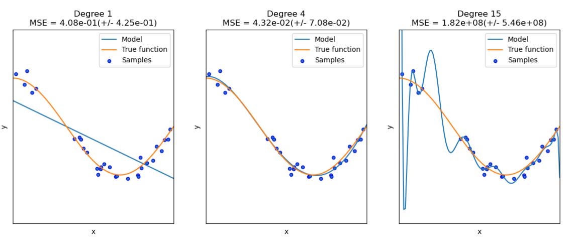
       评估过拟合还是欠拟合，一般有两种曲线类型，横坐标表示train_sizes，纵坐标有两种方式，一种是loss or Mean Squared Error（均方误差，越小，说明模型描述数据越精确）；另一种是accuracy, precision, recall, or F1 score，如果 training score 和 the validation score 都很低, 表明模型欠拟合；如果 training score 很高 而 the validation score很低, 则表明模型是过拟合的，二者都比较好则是适度拟合。

       1.Mean Squared Error的计算，MSE是指参数估计值与参数真实值之差的平方，用来评价数据的变化程度，值越小，说明预测模型描述实验数据具有越好的精度越。

'''查看均方误差MSE'''
mse_train = mean_squared_error(Y_train,y_train_v)
mse_test = mean_squared_error(Y_test,y_test_v)

print('mse_train:',mse_train)
print('mse_test:',mse_test)

mse_train: 0.15223333333333333
mse_test: 0.157175

       2.learning_curve展示了在训练期间添加更多训练样本呈现出的模型效果，通过检查模型在训练分数和测试分数方面的统计性能来描述效果。查看学习曲线，发现train score很高，test score较低，说明模型过拟合。

'''学习曲线查看拟合情况'''
import numpy as np
import matplotlib.pyplot as plt
from sklearn.model_selection import learning_curve
from sklearn.model_selection import ShuffleSplit
from sklearn.model_selection import LearningCurveDisplay

fig = plt.figure(figsize=(20,15))
cv= ShuffleSplit(n_splits=50,test_size=0.4,random_state=0)
train_sizes, train_scores, test_scores = learning_curve(model, X, target,cv=cv,n_jobs=4,)
train_scores_mean = np.mean(train_scores, axis=1)
test_scores_mean = np.mean(test_scores, axis=1)
train_scores_std = np.std(train_scores, axis=1)
test_scores_std = np.std(test_scores, axis=1)
plt.fill_between(train_sizes, train_scores_mean - train_scores_std,
                     train_scores_mean + train_scores_std, alpha=0.1,
                     color="r")
plt.fill_between(train_sizes, test_scores_mean - test_scores_std,
                     test_scores_mean + test_scores_std, alpha=0.1, color="g")
plt.plot(train_sizes,train_scores_mean,'o-',color="r",label='Train_score')
plt.plot(train_sizes,test_scores_mean,'o-',color="g",label = 'Test_score')
plt.xlabel('train sizes')
plt.ylabel('Accuracy')
plt.legend(loc='best')

plt.show()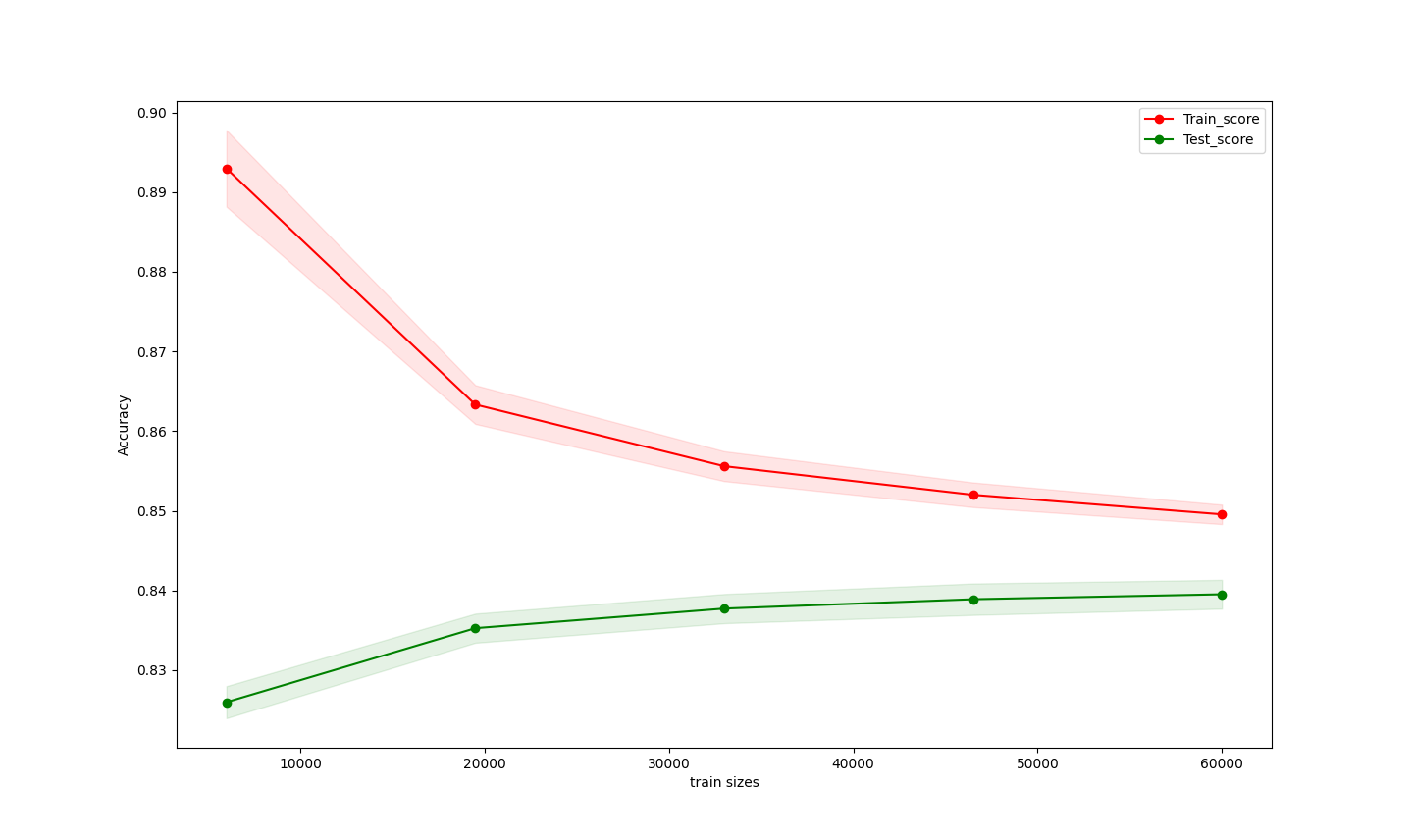

 三、模型过拟合参数调整 

1、使用较小的maxBin

2、使用较小的num_Leaves

3、使用minSumHessianInLeaf

4、通过设置baggingFraction和 baggingFreq来使用 bagging

5、通过设置 featureFraction来使用特征子抽样

6、增大训练数据集

7、使用lambdaL1, lambdaL2 来使用正则化

8、尝试maxDepth来避免生成过深的树

继续优化，后续文章写