Tensorflow—Neural Style Transfer

说明：本文章为作者在学习Tensorflow官方教程时的学习笔记，现整理出来供大家学习参考。您可以将本文章当作官方教程的中文翻译来阅读学习。本教程代码与官方代码一致，只有少许地方有细微改动。

Tensorflow官方教程链接附在文章末。

教程实际效果展示

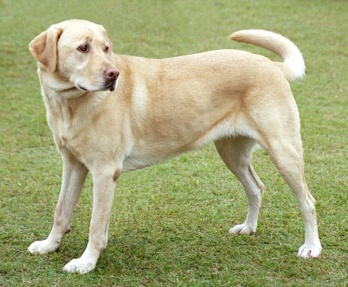
本教程将使用图片1与图片2生成图片3

图片1——内容图片¹

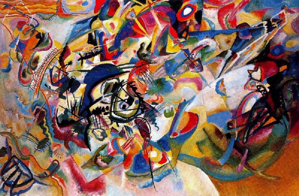
图片2——风格图片²

图片3——结果图片（参数设置 epoch=10, step_per_epoch=100）

风格迁移概述 & 本教程实现思路

风格迁移概述

图像经过卷积层之后得到的特征图的协方差矩阵可以很好的表征图像的纹理特征，但是会损失位置信息。但是在风格迁移的任务中，我们可以忽略位置信息损失这个缺点，只需要找到一个方法可以表征图像的纹理信息，并把这些纹理信息迁移到需要被风格迁移的图像中，完成风格迁移的任务。

在本教程中，我们使用克莱姆矩阵来代替协方差矩阵，它能够描述全局特征的自相关。

本教程实现思路

在本教程中，我们从已经训练好的图像分类网络VGG19 中挑选中间层来提取图像的纹理特征。

官方教程里还介绍了使用Tensorflow_Hub进行直接快速的风格迁移的例子，在本文中我们不过多赘述。

前期准备

软件准备

• 安装anaconda最新版本³，点击Download选择对应的版本下载即可；（建议使用GPU版本）
  作者的CPU为 Intel® Core™ i5-8300H CPU @ 2.30GHz 2.30 GHz
• 本教程使用Python 3.7.7版本
• 安装Tensorflow、Keras、Matplotlib、Numpy

数据准备（下载内容和风格图片）

content_path = tf.keras.utils.get_file('YellowLabradorLooking_new.jpg', 'https://storage.googleapis.com/download.tensorflow.org/example_images/YellowLabradorLooking_new.jpg')
style_path = tf.keras.utils.get_file('kandinsky5.jpg','https://storage.googleapis.com/download.tensorflow.org/example_images/Vassily_Kandinsky%2C_1913_-_Composition_7.jpg')

代码实现

导入相应模块

import os
import tensorflow as tf
# Load compressed models from tensorflow_hub
os.environ['TFHUB_MODEL_LOAD_FORMAT'] = 'COMPRESSED'

import IPython.display as display

import matplotlib.pyplot as plt
import matplotlib as mpl
mpl.rcParams['figure.figsize'] = (12, 12)
mpl.rcParams['axes.grid'] = False

import numpy as np
import PIL.Image
import time
import functools

def tensor_to_image(tensor): #定义张量到图像的变换函数
  tensor = tensor*255
  tensor = np.array(tensor, dtype=np.uint8)
  if np.ndim(tensor)>3:
    assert tensor.shape[0] == 1
    tensor = tensor[0]
  return PIL.Image.fromarray(tensor)

在屏幕上显示已经下载两张图片

• 定义一个函数来加载图片，并且将图片的最大尺寸限制在512像素。

def load_img(path_to_img):
  max_dim = 512
  img = tf.io.read_file(path_to_img)
  img = tf.image.decode_image(img, channels=3)
  img = tf.image.convert_image_dtype(img, tf.float32)

  shape = tf.cast(tf.shape(img)[:-1], tf.float32)
  long_dim = max(shape)
  scale = max_dim / long_dim

  new_shape = tf.cast(shape * scale, tf.int32)

  img = tf.image.resize(img, new_shape)
  img = img[tf.newaxis, :]
  return img

• 定义一个函数来显示图片

def imshow(image, title=None):
  if len(image.shape) > 3:
    image = tf.squeeze(image, axis=0)

  plt.imshow(image)
  if title:
    plt.title(title)

• 显示图像

content_image = load_img(content_path)
style_image = load_img(style_path)

plt.subplot(1, 2, 1)
imshow(content_image, 'Content Image')

plt.subplot(1, 2, 2)
imshow(style_image, 'Style Image')

现在两张图片应该显示在了你的屏幕上

定义内容和风格表现

我们可以使用模型的中间层来获取图片的内容和风格表现。

从网络的输入层开始，最开始的几层可以用来表示边缘和纹理这样的低级特征。当你逐步浏览网络，最后几层可以用来表示图像的高级特征——如轮子或者眼睛。

在本教程中，我们使用VGG19网络架构的中间层来定义图像的内容和风格表现，尝试在这些中间层上匹配相应的样式和内容目标表示。

• 加载一个不包含分类头的VGG19，并列出它的层名

vgg = tf.keras.applications.VGG19(include_top=False, weights='imagenet')
#如果你想要加载分类头，可以把上面的 False改为 True
print()
for layer in vgg.layers:
  print(layer.name)

• 从网络中选择中间层来表现图片的内容和风格

content_layers = ['block5_conv2'] 

style_layers = ['block1_conv1',
                'block2_conv1',
                'block3_conv1', 
                'block4_conv1', 
                'block5_conv1']

num_content_layers = len(content_layers)
num_style_layers = len(style_layers)

为什么这些中间输出层可以定义图片的内容和风格表示

在高层特征中，一个网络想要实现图像分类，那么它就必须要理解图片。这就要求将原始图像作为输入像素，并建立一个内部表示，将原始图像像素转换为对应图像内特征的复杂理解。

这也是为什么卷积神经网络可以有较好效果的一个原因：它们能够捕捉不受背景噪音和其他干扰影响的类的不变性和定义特征。

所以当图像输入到模型中，此时模型充当一个复杂的特征提取器。通过访问模型的中间层，我们就能够描述输入图像的内容和样式。

建立模型

• 该网络设计在tf.keras.applications中，我们可以通过Keras functional API提取中间层的的值。
• 我们可以使用model = Model(inputs, outputs)来定义模型。

下面的函数可以构建一个返回中间层输出列表的VGG19模型

def vgg_layers(layer_names):
  """ Creates a vgg model that returns a list of intermediate output values."""
  # Load our model. Load pretrained VGG, trained on imagenet data
  vgg = tf.keras.applications.VGG19(include_top=False, weights='imagenet')
  vgg.trainable = False

  outputs = [vgg.get_layer(name).output for name in layer_names]

  model = tf.keras.Model([vgg.input], outputs)
  return model

style_extractor = vgg_layers(style_layers)
style_outputs = style_extractor(style_image*255)

#Look at the statistics of each layer's output
for name, output in zip(style_layers, style_outputs):
  print(name)
  print("  shape: ", output.numpy().shape)
  print("  min: ", output.numpy().min())
  print("  max: ", output.numpy().max())
  print("  mean: ", output.numpy().mean())
  print()

计算风格（计算克莱姆矩阵）

通过在每个位置取特征向量与自身的外积，并在所有位置上求该外积的平均值，计算包含此信息的克莱姆矩阵。

这个可以使用tf.linalg.einsum函数来实现

def gram_matrix(input_tensor):
  result = tf.linalg.einsum('bijc,bijd->bcd', input_tensor, input_tensor)
  input_shape = tf.shape(input_tensor)
  num_locations = tf.cast(input_shape[1]*input_shape[2], tf.float32)
  return result/(num_locations)

提取图像的风格和内容

建立一个返回风格和内容张量的模型

class StyleContentModel(tf.keras.models.Model):
  def __init__(self, style_layers, content_layers):
    super(StyleContentModel, self).__init__()
    self.vgg = vgg_layers(style_layers + content_layers)
    self.style_layers = style_layers
    self.content_layers = content_layers
    self.num_style_layers = len(style_layers)
    self.vgg.trainable = False

  def call(self, inputs):
    "Expects float input in [0,1]"
    inputs = inputs*255.0
    preprocessed_input = tf.keras.applications.vgg19.preprocess_input(inputs)
    outputs = self.vgg(preprocessed_input)
    style_outputs, content_outputs = (outputs[:self.num_style_layers],
                                      outputs[self.num_style_layers:])

    style_outputs = [gram_matrix(style_output)
                     for style_output in style_outputs]

    content_dict = {content_name: value
                    for content_name, value
                    in zip(self.content_layers, content_outputs)}

    style_dict = {style_name: value
                  for style_name, value
                  in zip(self.style_layers, style_outputs)}

    return {'content': content_dict, 'style': style_dict}

extractor = StyleContentModel(style_layers, content_layers)

results = extractor(tf.constant(content_image))

当我们输入图像之后，该模型将会返回style_layers的克莱姆矩阵和content_layers的内容。

运行梯度下降

有了风格和内容提取器，我们现在可以运行风格迁移算法程序。

通过计算图像输出相对于每个目标的均方误差，然后取这些损失的加权和。

建立风格和内容目标值

style_targets = extractor(style_image)['style']
content_targets = extractor(content_image)['content']

定义一个tf.Variable来包含要优化的图像。在文章之前的代码中已经将图片的像素值设为了float32型。（tf.Variable必须和内容图像有相同的形状）

为了让算法更快，我们将图片的像素值限制在0到1之间

image = tf.Variable(content_image)

def clip_0_1(image):
  return tf.clip_by_value(image, clip_value_min=0.0, clip_value_max=1.0)

建立一个优化器，并使用两个损失的加权组合来得到总损失。

本教程中使用的时Adma，但推荐使用LBFGS。

opt = tf.optimizers.Adam(learning_rate=0.02, beta_1=0.99, epsilon=1e-1)

style_weight=1e-2
content_weight=1e4

def style_content_loss(outputs):
    style_outputs = outputs['style']
    content_outputs = outputs['content']
    style_loss = tf.add_n([tf.reduce_mean((style_outputs[name]-style_targets[name])**2) 
                           for name in style_outputs.keys()])
    style_loss *= style_weight / num_style_layers

    content_loss = tf.add_n([tf.reduce_mean((content_outputs[name]-content_targets[name])**2) 
                             for name in content_outputs.keys()])
    content_loss *= content_weight / num_content_layers
    loss = style_loss + content_loss
    return loss

使用tf,GradientTape来更新图片

@tf.function()
def train_step(image):
  with tf.GradientTape() as tape:
    outputs = extractor(image)
    loss = style_content_loss(outputs)

  grad = tape.gradient(loss, image)
  opt.apply_gradients([(grad, image)])
  image.assign(clip_0_1(image))

现在我们可以试着运行几次来测试我们的程序

train_step(image)
train_step(image)
train_step(image)
tensor_to_image(image)

输出结果：

接着我们再运行多次，以获取更好的效果

import time
start = time.time()

epochs = 10
steps_per_epoch = 100

step = 0
for n in range(epochs):
  for m in range(steps_per_epoch):
    step += 1
    train_step(image)
    print(".", end='', flush=True)
  display.clear_output(wait=True)
  display.display(tensor_to_image(image))
  print("Train step: {}".format(step))

end = time.time()
print("Total time: {:.1f}".format(end-start))

进行这一步的读者如果使用的是CPU版本的话，出结果的速度会比较慢，可以将epochs或者step_per_epoch的值设低一些。

输出结果：

• 本教程到这里就结束了，在官方教程⁴里还有后续的优化，有兴趣的读者可以点击下面的链接。

谢谢观看！！！

---

1. 内容图片的URL ↩︎

2. 风格图片的URL ↩︎

3. anaconda官网 ↩︎

4. 官方教程 ↩︎