强化学习笔记（5）价值估计函数Value Function Approximation

Introduction

之前所使用的算法一般都是使用字典或者查表的方法才存储价值函数。

• 每一个状态都有一个V(s)
• 每一个状态行为价值对都有一个Q(s,a)

在处理大规模的MDPs问题时，有很多状态或者行为需要存储在内存中，去查找和存储的开销特别大。

如何解决这种大规模的MDPs问题呢？如果有一个估计价值的函数，那么就用存储了，现用现算

• 使用Estimate value function 来估计状态价值。

$$\begin{gathered} \hat{v}(s,w)\approx v_{\pi }(s) \\ or\hat{q}(s,a,w)\approx q_{\pi }(s,a) \end{gathered}$$

w是一个参数，通过MC或者TD学习来更新它。通过调整w，使得估计出来的和实际的近似。

从可见的状态可以推广到不可见的状态。

通过Estimate value function , 那么强化学习的任务就转变成了求解近似参数w的问题了。

如何选择Function Approximator?

有许多function approximators, 例如：

• Linear combination of features;
• Neural network;
• Decision tree;
• Nearest neighbour;
• Fourier / wavelet bases;
• …

Incremental Methods

我们问题转化成了求解进近似参数w。

Gradient Descent

设$J(w)$是w的cost function，代表w和最理想的值之间的差距。使用梯度下降的方法逼近最优w。
$$\begin{array}{rl}J(w)& =\frac{1}{2}{\mathbb{E}}_{\pi }[(v_{\pi }(s)-\hat{v}(s,w){)}^2]\\ & =\frac{1}{2n}\sum _{i=1}^n(v_{\pi }(s{)}^{(i)}-\hat{v}(s,w{)}^{(i)}{)}^{2}i代表第i个example\end{array}$$

$v_{\pi }(s)$是实际的值

$\hat{v}(s,w)$是估计的值

J(w)是实际的值与估计值偏差平方 的数学期望。 （最小二乘法）

乘以1/2是为了求偏导消去产生的2

梯度的方向是$J(w)$上升速度最快的方向。（其实是把上升速度最快的方向定义成了梯度）

J(w)的梯度：就是对w里的每个维度都求偏导。

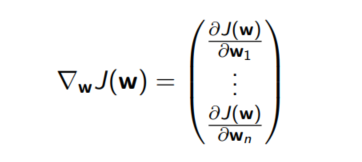
我们想让J(w)不断迭代变小，就需要使用梯度的反方向，也就是下降最快的方向。

每次w更新的大小（$w\leftarrow w+△w$）：
$$\begin{gathered} △w=\alpha {\nabla }_{w}J(w) \\ =\alpha {\mathbb{E}}_{\pi }[(v_{\pi }(S)-\hat{v}(S,w)){\nabla }_w\hat{v}(S,w)] \\ =\alpha \frac{1}{n}\sum _{i=1}^n(v_{\pi }(S{)}^{(i)}-\hat{v}(S,w{)}^{(i)}){\nabla }_w\hat{v}(S,w{)}^{(i)} \end{gathered}$$

$\alpha$是步长

i是第i个example

以上的公式由于需要求数学期望，在内存中，在更新某一个维度的信息时，需要存储所有的n个example的信息。

数学期望 = 试验中每次可能结果的概率乘以其结果的总和。

随机梯度下降(Stochastic gradient)解决了每次迭代需要存储所有example的信息的问题。为大规模的高纬度训练提供了可能。每次迭代只使用一个example。
$$△\mathbf{w}=\alpha ({\mathbf{v}}_{\pi }(\mathbf{S})-\hat{\mathbf{v}}(\mathbf{S},\mathbf{w})){\nabla }_{\mathbf{w}}\hat{\mathbf{v}}(\mathbf{S},\mathbf{w})$$
还有介于两者之间的批量梯度下降。batch- gradient

特征向量的形式

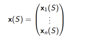
Linear Value Function Approximation线性价值估计函数

使用线性函数来估计价值：
$$\hat{v}(S,w)=\mathbf{x}(\mathbf{S}{)}^{\mathbf{T}}w=\sum _{\mathbf{j}=1}^{\mathbf{n}}{\mathbf{x}}_{\mathbf{j}}(\mathbf{S}){\mathbf{w}}_{\mathbf{j}}$$
以w为参数变量的目标函数(此处可以乘1/2)
$$J(\mathbf{w})={\mathbb{E}}_{\pi }[({\mathbf{v}}_{\pi }(\mathbf{S})-\mathbf{x}(\mathbf{S}{)}^{\mathbf{T}}\mathbf{w}{)}^2]$$
根据随机前面梯度下降（Stochastic gradient descent）更新规则：

$△w=\alpha (v_{\pi }(S)-\hat{v}(S,w)){\nabla }_w\hat{v}(S,w)$

• $\hat{v}$的梯度：${\nabla }_{\mathbf{w}}\hat{v}(S,\mathbf{w})=\mathbf{x}(\mathbf{S})$

• w的更新量： $△\mathbf{w}=\alpha ({\mathbf{v}}_{\pi }(\mathbf{S})-\hat{\mathbf{v}}(\mathbf{S},\mathbf{w}))\ast \mathbf{x}(\mathbf{S})$

正确结果

使用supervised learning方法来近似，然而我们并不知道target： $v_{\pi }(S)$。在RL中只有奖励。

在实际应用中，我们使用其他来代替target。
$$△\mathbf{w}=\alpha (\mathbf{t}\mathbf{a}\mathbf{r}\mathbf{g}\mathbf{e}\mathbf{t}-\hat{\mathbf{v}}({\mathbf{S}}_{\mathbf{t}},\mathbf{w})){\nabla }_{\mathbf{w}}\hat{\mathbf{v}}({\mathbf{S}}_{\mathbf{t}},\mathbf{w})$$

• 对于MC类，target是return（收获）$G_t$

  • MC算法收敛到局部最优解。即使使用非线性的估计函数
  • $G_t$是无偏差的

• 对于TD(0)，target是TD target： $R_{t+1}+\gamma \hat{v}(S_{t+1},\mathbf{w})$

  • TD-target 和最优价值函数$v_\pi(S) $是有偏差的，但应用在此处效果也很好。
  • TD(0)收敛于（接近）全局最优

• 对于$TD(\lambda )$, target是$\lambda$-return(收获) $G_t^{\lambda }$

  • $\lambda -return$ $G_t^{\lambda }$也是和真正的$v_{\pi }(S)$有偏差，可以应用于训练数据
    

Batch Methods

• 梯度下降简单易用，但是没有充分利用采样
• Batch Methods为了根据所给的agent的经验，从而找到最适合的value function

Least Squares Prediction

Experience Replay

给出一些列的状态价值对：
D = { < s 1 , v 1 > , . . . . < s T , v T > } \mathcal D = \{<s_1, v_1>, .... <s_T,v_T>\} D={<s1​,v1​>,....<sT​,vT​>}
重复以下步骤：

1. 选取从经验中选取一定数量的 <state,value>

2. 使用随机梯度算法来更新参数
   $$△\mathbf{w}=\alpha ({\mathbf{v}}_{\pi }(\mathbf{S})-\hat{\mathbf{v}}(\mathbf{S},\mathbf{w})){\nabla }_{\mathbf{w}}\hat{\mathbf{v}}(\mathbf{S},\mathbf{w})$$

可以收敛到最小二乘法的解
$${\mathbf{w}}^{\pi }=\arg mi{n}_{\mathbf{w}}LS(\mathbf{w})$$

DQN (Deep Q-Networks)

Q-learning更新公式：
$$Q(S_t,A_t)\leftarrow Q(S_t,A_t)+\alpha (R_{t+1}+\gamma Q(S_{t+1},A^{\prime })-Q(S_t,A_t))$$

A’是根据借鉴策略来的。

借鉴策略如果是贪婪策略，那么可化简：
$$Q(S_t,A_t)\leftarrow Q(S_t,A_t)+\alpha (R_{t+1}+\gamma \underset{a^{\prime }}{\max }Q(S_{s+1},a^{\prime })-Q(S_t,A_t))$$

$\alpha$： 学习率，决定每次的更新量。$\alpha$过小，会导致过于注重之前的知识，导致学习的太慢。过大，则会导致过于在乎新的学习，忘记之前的经验积累。

$\gamma$：预测出来的下一个状态Q值对当前的影响。范围(0,1)

如果 $ \alpha = 1$ ，那么上式(这一步的推导和贝尔曼方程有关)
$$Q(S_t,A_t)\leftarrow R_{t+1}+\gamma \underset{a^{\prime }}{\max }Q(S_{s+1},a^{\prime })$$
这就是我们每次的Q值更新公式。我们的需要一个网络能够拟合出这个Q值的计算过程。这个网络的输入参数为state，输出参数为每个action在该状态下的Q值。这个网络就是Q网络。

当然，我们在训练时，每次的迭代目标target就是通过上式计算出来的。我们希望网络产生的数据和我们target相同
$$target=R_{t+1}+\gamma \arg \max Q(S_{t+1},a)$$

一些DQN的升级

Nature DQN

可以理解成两个网络Q和Q‘

Q负责产生动作。Q’负责在训练(replay)Q时，计算target值。Q’ 的权重是直接从Q中复制过来的。自己本省不进行训练。

Double DQN

为了解决Over Estimate问题。这个问题的根源是因为使用贪婪算法。

有两个Q网络。一个立刻更新，一个延迟更新。

Dueling DQN

相比Double DQN，后面多了两个子网络，分别对应价值函数部分和优势函数部分。然后累加得到输出层。

使用Huber loss

是一个带参数的损失函数，和之前的用的均方误差损失函数（MSE, mean square error）相比，对于噪声（离群点）不敏感。所以有很好的适应性。

计算公式
$$L_{\delta }=\{\begin{array}{l}\frac{1}{2}{e}^2,|e|\le \delta \\ \delta (|e|-\frac{1}{2}\delta ),otherwise\end{array}$$

e是预测值与target之间的偏差。

$\delta$是一个界限