Tensorflow学习笔记：基础篇（8）——Mnist手写集改进版（过拟合与Dropout）

最新推荐文章于 2021-03-31 15:08:03 发布

Laurenitum

最新推荐文章于 2021-03-31 15:08:03 发布

阅读量1.1k

点赞数 2

分类专栏： Tensorflow学习笔记

本文链接：https://blog.csdn.net/Laurenitum0716/article/details/78992676

版权

Tensorflow学习笔记专栏收录该内容

20 篇文章 5 订阅

订阅专栏

Tensorflow学习笔记：基础篇（8）——Mnist手写集改进版（过拟合与Dropout）

前序

— 前文中，我们在三层全连接神经网络中使用了Tensorboard对模型训练中的参数与模型架构进行可视化显示
— 本文我们来说一个相对简单的问题：过拟合
Reference：正则化方法：L1和L2 regularization、数据集扩增、dropout，什么是过拟合？

过拟合

— 在机器学习中，我们提高了在训练数据集上的表现力时，在测试数据集上的表现力反而下降了，这就是过拟合。
— 过拟合发生的本质原因，是由于监督学习的不适定性。比如我们再学习线性代数时，给出n个线性无关的方程，我们可以解出来n个变量，但是肯定解不出来n+1个变量。在机器学习中，如果数据（对应于方程）远小于模型空间（对应求解的变量），那么，就容易发生过拟合现象。

解决过拟合的三种方式：
（1）增加训练数据集
（2）正则化
（3）Dropout

Dropout

正则化是通过修改代价函数来实现的，而Dropout则是通过修改神经网络本身来实现的，它是在训练网络时用的一种技巧。
这里写图片描述
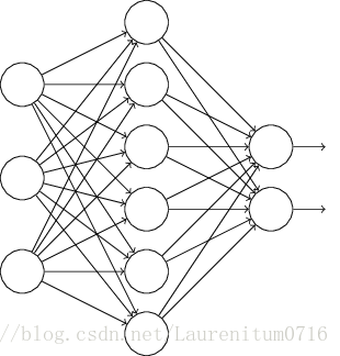
假设我们要训练上图这个网络，在训练开始时，我们随机地“删除”一半的隐层单元，视它们为不存在，得到如下的网络：

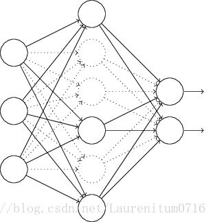
保持输入输出层不变，按照BP算法更新上图神经网络中的权值（虚线连接的单元不更新，因为它们被“临时删除”了）。

以上就是一次迭代的过程，在第二次迭代中，也用同样的方法，只不过这次删除的那一半隐层单元，跟上一次删除掉的肯定是不一样的，因为我们每一次迭代都是“随机”地去删掉一半。第三次、第四次……都是这样，直至训练结束。

以上就是Dropout，它为什么有助于防止过拟合呢？可以简单地这样解释，运用了dropout的训练过程，相当于训练了很多个只有半数隐层单元的神经网络（后面简称为“半数网络”），每一个这样的半数网络，都可以给出一个分类结果，这些结果有的是正确的，有的是错误的。随着训练的进行，大部分半数网络都可以给出正确的分类结果，那么少数的错误分类结果就不会对最终结果造成大的影响。

代码示例

1、数据准备

import tensorflow as tf
from tensorflow.examples.tutorials.mnist import input_data

# 载入数据集
mnist = input_data.read_data_sets("MNIST_data", one_hot=True)

# 每个批次送100张图片
batch_size = 100
# 计算一共有多少个批次
n_batch = mnist.train.num_examples // batch_size

def variable_summaries(var):
    with tf.name_scope('summaries'):
        mean = tf.reduce_mean(var)
        tf.summary.scalar('mean', mean)
        with tf.name_scope('stddev'):
            stddev = tf.sqrt(tf.reduce_mean(tf.square(var - mean)))
        tf.summary.scalar('stddev', stddev)
        tf.summary.scalar('max', tf.reduce_max(var))
        tf.summary.scalar('min', tf.reduce_min(var))
        tf.summary.histogram('histogram', var)  ##直方图

2、准备好placeholder

我们今天新建一个placeholder，取名为keep_prob，它的作用是控制实际参与训练的神经元比例，取值范围为0.0-1.0，若取1.0，表示100%神经元参与训练；若取0.6，表示60%神经元工作，以此类推。

with tf.name_scope('input'):
    x = tf.placeholder(tf.float32, [None, 784], name='x_input')
    y = tf.placeholder(tf.float32, [None, 10], name='y_input')
    keep_prob = tf.placeholder(tf.float32, name='keep_prob')
    lr = tf.Variable(0.001, dtype=tf.float32, name='learning_rate')

3、初始化参数/权重

这里我们使用tf.nn.dropout(）函数来实现Dropout，通过keep_prob参数控制

with tf.name_scope('layer'):
    with tf.name_scope('Input_layer'):
        with tf.name_scope('W1'):
            W1 = tf.Variable(tf.truncated_normal([784, 500], stddev=0.1), name='W1')
            variable_summaries(W1)
        with tf.name_scope('b1'):
            b1 = tf.Variable(tf.zeros([500]) + 0.1, name='b1')
            variable_summaries(b1)
        with tf.name_scope('L1'):
            L1 = tf.nn.tanh(tf.matmul(x, W1) + b1, name='L1')
        L1_drop = tf.nn.dropout(L1, keep_prob)
    with tf.name_scope('Hidden_layer'):
        with tf.name_scope('W2'):
            W2 = tf.Variable(tf.truncated_normal([500, 300], stddev=0.1), name='W2')
            variable_summaries(W2)
        with tf.name_scope('b2'):
            b2 = tf.Variable(tf.zeros([300]) + 0.1, name='b2')
            variable_summaries(b2)
        with tf.name_scope('L2'):
            L2 = tf.nn.tanh(tf.matmul(L1_drop, W2) + b2, name='L2')
        L2_drop = tf.nn.dropout(L2, keep_prob)
    with tf.name_scope('Output_layer'):
        with tf.name_scope('W3'):
            W3 = tf.Variable(tf.truncated_normal([300, 10], stddev=0.1), name='W3')
            variable_summaries(W3)
        with tf.name_scope('b3'):
            b3 = tf.Variable(tf.zeros([10]) + 0.1, name='b3')
            variable_summaries(b3)

4、计算预测结果

prediction = tf.nn.softmax(tf.matmul(L2, W3) + b3)

5、计算损失值

with tf.name_scope('loss'):
    loss = tf.reduce_mean(tf.nn.softmax_cross_entropy_with_logits(labels=y, logits=prediction))
    tf.summary.scalar('loss', loss)

6、初始化optimizer

with tf.name_scope('optimizer'):
    optimizer = tf.train.AdamOptimizer(lr).minimize(loss)

with tf.name_scope('train'):
    with tf.name_scope('correct_prediction'):
        correct_prediction = tf.equal(tf.argmax(y, 1), tf.argmax(prediction, 1))

    with tf.name_scope('accuracy'):
        accuracy = tf.reduce_mean(tf.cast(correct_prediction, tf.float32))
        tf.summary.scalar('accuracy', accuracy)

7、指定迭代次数，并在session执行graph

init = tf.global_variables_initializer()
merged = tf.summary.merge_all()


with tf.Session() as sess:
    sess.run(init)
    writer = tf.summary.FileWriter('./graphs/mnist', sess.graph)

    for epoch in range(21):
        sess.run(tf.assign(lr, 0.001 * (0.95 ** epoch)))
        for batch in range(n_batch):
            batch_xs, batch_ys = mnist.train.next_batch(batch_size)
            summary, _ = sess.run([merged, optimizer], feed_dict={x: batch_xs, y: batch_ys, keep_prob: 1.0})
            #这里同样将keep_prob使用字典形式传入，我们分别取0.6和1.0，运行两次，比较结果
        writer.add_summary(summary, epoch)
        test_acc = sess.run(accuracy, feed_dict={x: mnist.test.images, y: mnist.test.labels, keep_prob: 1.0})
        train_acc = sess.run(accuracy, feed_dict={x: mnist.train.images, y: mnist.train.labels, keep_prob: 1.0})
        #这里我们分别让它同时运行测试集与训练集，同时输出准确率进行比较，执行测试时，我们将keep_prob取为1，让神经元全部工作。
        learning_rate = sess.run(lr)
        if epoch % 2 == 0:
            print("Iter" + str(epoch) + ", Testing accuracy:" + str(test_acc) + ", Training accuracy:" + str(train_acc))

    writer.close()

运行结果

我们先将keep_prob设置为1.0训练模型，得到下图，发现Testing accuracy依然为0.98，Training accuracy达到0.996，这也不难理解，比较用training的数据集训练的模型，拿来测试自身的准确度肯定是很高的。
但是，我想请各位读者注意的是，Testing accuracy与Training accuracy的差值随着迭代次数增加，而逐渐扩大，说明产生了文章开头提到过拟合现象，即在训练数据集上的表现力时，在测试数据集上的表现力反而下降了。
这里写图片描述
我们再来看keep_prob设置为0.6的运行结果：

大家可以发现，Testing accuracy与Training accuracy较之前均有所下降，但是其之间的差值较之前有所改善，说明使用Dropout能够在一定程度上缓解过拟合现象，大家不妨尝试将keep_prob多取几个值进行比较一下~~

完整代码

import tensorflow as tf
from tensorflow.examples.tutorials.mnist import input_data

mnist = input_data.read_data_sets("MNIST_data", one_hot=True)

# 每个批次的大小
batch_size = 100
# 计算一共有多少个批次
n_batch = mnist.train.num_examples // batch_size


def variable_summaries(var):
    with tf.name_scope('summaries'):
        mean = tf.reduce_mean(var)
        tf.summary.scalar('mean', mean)
        with tf.name_scope('stddev'):
            stddev = tf.sqrt(tf.reduce_mean(tf.square(var - mean)))
        tf.summary.scalar('stddev', stddev)
        tf.summary.scalar('max', tf.reduce_max(var))
        tf.summary.scalar('min', tf.reduce_min(var))
        tf.summary.histogram('histogram', var)  ##直方图


with tf.name_scope('input'):
    x = tf.placeholder(tf.float32, [None, 784], name='x_input')
    y = tf.placeholder(tf.float32, [None, 10], name='y_input')
    keep_prob = tf.placeholder(tf.float32, name='keep_prob')
    lr = tf.Variable(0.001, dtype=tf.float32, name='learning_rate')

with tf.name_scope('layer'):
    with tf.name_scope('Input_layer'):
        with tf.name_scope('W1'):
            W1 = tf.Variable(tf.truncated_normal([784, 500], stddev=0.1), name='W1')
            variable_summaries(W1)
        with tf.name_scope('b1'):
            b1 = tf.Variable(tf.zeros([500]) + 0.1, name='b1')
            variable_summaries(b1)
        with tf.name_scope('L1'):
            L1 = tf.nn.tanh(tf.matmul(x, W1) + b1, name='L1')
        L1_drop = tf.nn.dropout(L1, keep_prob)
    with tf.name_scope('Hidden_layer'):
        with tf.name_scope('W2'):
            W2 = tf.Variable(tf.truncated_normal([500, 300], stddev=0.1), name='W2')
            variable_summaries(W2)
        with tf.name_scope('b2'):
            b2 = tf.Variable(tf.zeros([300]) + 0.1, name='b2')
            variable_summaries(b2)
        with tf.name_scope('L2'):
            L2 = tf.nn.tanh(tf.matmul(L1_drop, W2) + b2, name='L2')
        L2_drop = tf.nn.dropout(L2, keep_prob)
    with tf.name_scope('Output_layer'):
        with tf.name_scope('W3'):
            W3 = tf.Variable(tf.truncated_normal([300, 10], stddev=0.1), name='W3')
            variable_summaries(W3)
        with tf.name_scope('b3'):
            b3 = tf.Variable(tf.zeros([10]) + 0.1, name='b3')
            variable_summaries(b3)
        prediction = tf.nn.softmax(tf.matmul(L2_drop, W3) + b3)

# 二次代价函数
# loss = tf.reduce_mean(tf.square(y - prediction))

# 交叉熵代价函数
with tf.name_scope('loss'):
    loss = tf.reduce_mean(tf.nn.softmax_cross_entropy_with_logits(labels=y, logits=prediction))
    tf.summary.scalar('loss', loss)

# 梯度下降
# optimizer = tf.train.GradientDescentOptimizer(learning_rate).minimize(loss)
with tf.name_scope('optimizer'):
    optimizer = tf.train.AdamOptimizer(lr).minimize(loss)

with tf.name_scope('train'):
    with tf.name_scope('correct_prediction'):
        correct_prediction = tf.equal(tf.argmax(y, 1), tf.argmax(prediction, 1))

    with tf.name_scope('accuracy'):
        accuracy = tf.reduce_mean(tf.cast(correct_prediction, tf.float32))
        tf.summary.scalar('accuracy', accuracy)

merged = tf.summary.merge_all()

init = tf.global_variables_initializer()

with tf.Session() as sess:
    sess.run(init)
    writer = tf.summary.FileWriter('./graphs/mnist', sess.graph)

    for epoch in range(21):
        sess.run(tf.assign(lr, 0.001 * (0.95 ** epoch)))
        for batch in range(n_batch):
            batch_xs, batch_ys = mnist.train.next_batch(batch_size)
            summary, _ = sess.run([merged, optimizer], feed_dict={x: batch_xs, y: batch_ys, keep_prob: 0.6})

        writer.add_summary(summary, epoch)
        test_acc = sess.run(accuracy, feed_dict={x: mnist.test.images, y: mnist.test.labels, keep_prob: 1.0})
        train_acc = sess.run(accuracy, feed_dict={x: mnist.train.images, y: mnist.train.labels, keep_prob: 1.0})
        learning_rate = sess.run(lr)
        if epoch % 2 == 0:
            print("Iter" + str(epoch) + ", Testing accuracy:" + str(test_acc) + ", Training accuracy:" + str(train_acc))

    writer.close()

Laurenitum

关注

2
点赞
踩
4

收藏

觉得还不错? 一键收藏
0
评论
Tensorflow学习笔记：基础篇（8）——Mnist手写集改进版（过拟合与Dropout）

Tensorflow学习笔记：基础篇（8）——Mnist手写集改进版（过拟合与Dropout）前序— 前文中，我们在三层全连接神经网络中使用了Tensorboard对模型训练中的参数与模型架构进行可视化显示 — 本文我们来说一个相对简单的问题：过拟合 Reference：正则化方法：L1和L2 regularization、数据集扩增、dropout，什么是过拟合？过拟...
复制链接

扫一扫