


The study of momentum and oscillators is the analysis of price changes rather than price levels. Among technicians, momentum establishes the speed of price movement and the rate of ascent or descent.动量决定了价格变动的速度和上升或下降的速度 Analysts use momentum interchangeably with slope, the angle of inclination of price movement 斜率是价格变动的倾斜角度usually found with a simple least squares regression (Figure 9.1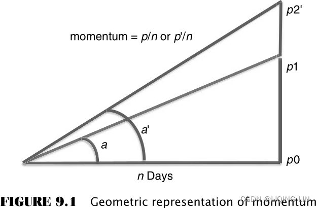 a pure momentum oscillator that measures the percent change in price from one period to the next). In mathematics it is also the first difference, the difference between today’s price and the previous day. Momentum is often considered using terms of Newton’s Law, which can be restated loosely as once started, prices tend to remain in motion in more-or-less the same direction.
Indicators of change, such as momentum and oscillators, are used as leading indicators of price direction. They can identify when the current trend is no longer maintaining its same level of strength; that is, they show when an upwards move is decelerating. Prices are rising, but at a slower rate. This gives traders an opportunity to begin liquidating their open trend trades before prices actually reverse. As the time period for the momentum calculation shortens, this indicator becomes more sensitive to small changes in price. It is often used in countertrend, or mean reversion strategy. The change in momentum, also called rate of change, acceleration, or second difference, is even more sensitive and anticipates change sooner.
Before beginning a discussion of various momentum calculations, a brief comment on terminology is necessary to understand how various techniques are grouped together. The use of a single price, such as Microsoft at $25.50 or gold at $1400, has no direction or movement implied. We are simply relating a price level and not indicating that prices are going up or down.
Next, we describe the speed at which prices are rising or falling. To know the speed, it is not enough to say that the S&P rose 3 points; you must specify the time interval over which this happened—“the S&P rose 3 points in 1 hour.” When you say that you drove your car at 60, you really imply that you were going 60 miles per hour, or 60 kilometers per hour. This description of speed, or distance covered over time, is the same information that is given by a single momentum value. Then, if the daily momentum of the NASDAQ 100 is +10, it is rising at the rate of 10 points per day.
Having made a point of saying that momentum is change over time, which it is, the “industry” uses momentum to mean price change with the time implied (and often not even given) where speed is always the price change divided by the time interval. The same interpretation will be used here. The term rate of change (ROC) will also be used to describe acceleration, an increase or decrease in the speed; when the rate of change is zero, we are talking about speed and momentum(Be careful about terminology. Many books and software use rate of change (ROC) interchangeably with momentum, the change in price over n days, rather than the change in momentum. Also, momentum indicators can also be used for mean reversion and may be called oscillators because their values swing from positive to negative.).
You will see in this chapter that acceleration is more sensitive than speed. We will begin with the least sensitive indicator, momentum, increase to acceleration, and then address the variations and applications, including divergence, the most popular use of momentum indicators.
MOMENTUM
Momentum is the difference between two prices taken over a fixed interval. It is an other word for speed, the distance covered over time; however, everyone uses it to mean change. For example, today’s 5-day momentum value would be the difference between M today’s price
 and the price five days ago:
- 5-day momentum,
- Using notation familiar to many programmers: 5-day momentum = price − price[5]
- or n-day momentum = price − price[n]
- where the notation [n] refers to the price n days ago.
The momentum value increases
![]() as the change in price
as the change in price![]() increases over the same 5-day period. Figure 9.1 shows how the momentum changes
increases over the same 5-day period. Figure 9.1 shows how the momentum changes![]() as the price increases
as the price increases![]() over the same time period.
over the same time period.
- Over n days, the price moves from
to
. It forms angle a and has a momentum of
.
For example, if the 5-day change in price is an increase of 100, then the momentum is simply 100, but the speed is 100/5 = 20.
 - If prices had increased to point , then the momentum would have been greater, and the angle a′ would have been larger.
If prices increase by 100 points over a 10-day time interval, the momentum would still be 100, but the speed, or slope, would be 100/10 = 10. - When calculating momentum, the interval of the calculation must always be stated. To avoid confusion, we state that the 5-day momentum is 20 and the 10-day momentum is 10.
Today’s 5-day momentum, which we will now show as can range in value from the maximum upwards move
![]() to the maximum downwards move
to the maximum downwards move![]() that the price can make in five days; the momentum is zero if prices are unchanged after five days. For stocks, there is no actual limit on the maximum price range over any time interval. In cases such as Enron, prices could collapse to zero in short order. From a practical view, most stocks and futures markets have a history of volatility that relates to their price level. The higher the price, the greater the price moves. As the price of gold rose to $1000 per ounce, the 5-day momentum could have been as high as $100 per ounce ($20 per day). When it was at $250 and investors lost interest, it may have shown a $1 per ounce change over five days.
that the price can make in five days; the momentum is zero if prices are unchanged after five days. For stocks, there is no actual limit on the maximum price range over any time interval. In cases such as Enron, prices could collapse to zero in short order. From a practical view, most stocks and futures markets have a history of volatility that relates to their price level. The higher the price, the greater the price moves. As the price of gold rose to $1000 per ounce, the 5-day momentum could have been as high as $100 per ounce ($20 per day). When it was at $250 and investors lost interest, it may have shown a $1 per ounce change over five days.
Momentum is not volatility. Gold can move from $1200 to $1250 in two days then back to $1200 over the next three days and the momentum would be zero but the volatility would be high.
 Figure 9.2 shows a typical pattern of momentum. Smooth prices are used to make the relationship between price change and momentum clear.
- During the first 15-day cycle, prices rise steadily, peaking on day 9.
- As prices rise at a slower rate during days 5 through 9 the momentum declines but remains above zero.
As long as the 5-day momentum is greater than zero, prices are rising. - The highest momentum
value occurs on day 3 when prices have the largest positive price change.
- On day 10 the momentum value is zero. Looking at the price chart, this occurs when the 5-day change in price is zero.
- The lowest momentum value occurs on day 16 when the prices have declined the most.
- After prices reach their lowest point and begin up, the momentum is negative but rising.
If prices always moved in the smooth pattern shown in Figure 9.2, then momentum would be a perfect leading indicator. You could buy when momentum turned up and sell when it turned down, and be ahead of the change in price direction. Unfortunately, prices movement is irregular; consequently, momentum values are irregular. Because momentum contains valuable information, we will look at a number of systematic ways to evaluate momentum and improve trading. These focus on extreme momentum values and momentum patterns, all of which have proved to be valuable additions to trading strategies, in particular to the timing of entries and exits.
Characteristics of Momentum
Momentum is a way of smoothing price movement and can serve the same purpose as a trend. Although the momentum values are not as smooth as a moving average, larger momentum periods reduce the extremes seen in the price chart. One key advantage of momentum is that it does not have the lag that exists in a moving average.

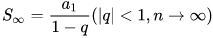
The AOL chart (Figure 9.3) compares 20- and 40-day moving averages at the top with 20- and 40-day momentum along the bottom. The 40-day momentum (dark line) is smoother and peaks at about the same place as the price. The faster 20-day momentum is not as smooth but peaks sooner than the 40-day momentum and actually leads the price movement. The peaks of the faster momentum represent the maximum price change over a 20-day period. Had prices continued higher at the same rate—that is, if prices had increased $1 per day—the 20-day momentum would have turned sideways and become a horizontal line.
The 20-day and 40-day momentum lines both peak significantly sooner than their moving average equivalents, showing that the speed represented by momentum is a more sensitive measure than the direction of a trendline. The cost of this leading indicator is the increased noise seen in the erratic pattern of momentum compared to the smoothness of the trendline.
Momentum can be used as a trend indicator by
- selling when the momentum value crosses downward through the horizontal line at zero
- and buying when it crosses above the zero line.
Because there is more noise in momentum than in the equivalent moving average, you would want to draw a small band around the zero line about the width of the small variations in momentum.
- A sell signal would be given when the momentum falls below the lower band and
- a buy when it moves upward through the upper band.
However, the momentum crossing zero is essentially the same as the moving average turning up or down. It means that the price today is the same as the price n-days ago. Chapter 8 compared the performance of a trend and a momentum system over the same calculation periods.
Momentum as a Percentage
It is always convenient to express all markets in the same notation. It makes comparisons much easier. For the stock market, momentum can be expressed as a percentage where a 1-day momentum is equivalent to the 1-day return,or, because they are returns, the alternative can be used, ln
. But momentum is most often calculated over more than one day; therefore, the n-day momentum as a percentage is
Using percentages does not work for futures markets because most data used for analysis are continuous, back-adjusted prices. Back-adjusting over many years and many contracts will cause the oldest data to be very different from the actual prices that occurred on those dates; therefore, percentages are incorrect. When using momentum with back-adjusted futures prices, it is best to use the price differences.
Momentum as the Difference between Price and Trend
The term momentum is very flexible. It is common for it to refer to the difference between today’s price and a corresponding moving average value, in a manner similar to beta, which indicates the relative strength of a stock compared to an index. The properties of this new value are the same as standard momentum.动量一词非常灵活。 它通常指的是今天的价格与相应的移动平均值之间的差异,其方式类似于 beta,表示股票与指数相比的相对强度。 这个新值的属性与标准动量相同
- As the momentum becomes larger, prices are moving away from the moving average.
- As it moves towards zero, the prices are converging with the moving average.
 FIGURE 9.4 Momentum is also called relative strength, the difference between two prices or a price and a moving average (lower panel). The traditional momentum calculation is shown in the center panel.
The upper panel of Figure 9.4 shows a 20-period moving average plotted on a daily chart of Intel during the 14 months ending May 2003.
- The center panel shows the standard 20-period momentum, the difference between prices that are 20 days apart.
- The range of values for the center panel is approximately +6 to −11
- The bottom panel is the difference between the price and the 20-day moving average.
- the scale on the lower panel is +3 to −7.
- Because a trendline lags behind price movement, the difference between the price and trendline is smaller at points where there are larger price swings 价格波动较大and typically larger momentum values(compare to the smallest negative momentum) 动量值通常较大.
A comparison of the two lower panels of Figure 9.4 also shows that there are differences in the small movements but the overall pattern is the same. When a price moves to an extreme, it is generally farthest from the moving average and farthest from the price n-days ago; therefore, the most extreme points occur at exactly the same place. This momentum calculation has also been called relative strength because it is measured relative to a previous price or relative to a trendline.
Momentum as a Trend Indicator
The momentum value is a smoothing of price changes and can serve the same purpose as a standard moving average. Many applications use momentum as a substitute for a price trend. By looking at the net change in price over the number of days designated by an n-day momentum indicator, intermediate fluctuations are ignored, and the pattern in price trend can be seen. The longer the span between the observed points, the momentum calculation period, the smoother the results. This is very similar to faster and slower moving averages.
In its simplest form, momentum is simply the difference between the current price and price of some fixed time periods in the past.
- Consecutive periods of positive momentum values indicate an uptrend;
- conversely, if momentum is consecutively negative, that indicates a downtrend.pa8_Contract for Difference CFD Trading_Oanda_git_log return_Momentum Strategy_Leverage_margin_tpqoa_LIQING LIN的博客-CSDN博客
To use momentum as a trend indicator, choose any calculation period.
- A buy signal occurs whenever the value of the momentum turns from negative to positive, and
- a sell signal is when the opposite occurs, as shown in Figure 9.5.
 FIGURE 9.5 Trend signals using momentum.
 - If a band is used to establish a neutral position or a commitment zone如果使用带来建立中性位置或保证(承诺)区, as discussed in the previous chapter, it should be drawn around the horizontal line representing the zero momentum value.
In order to find the best choice of a momentum span, a sampling of different values could be tested for optimum performance, or a chart could be examined for some natural price cycle.
- Identify the significant tops and bottoms of any bar chart, and average the number of days between these cycles,
- or find the number of days that would closely approximate the occurrences of these peaks and valleys. Then use ½ or ¼ the number of days from peak to peak or valley to valley. These natural cycles will often be the best choice of momentum calculation interval (Figure 9.6).
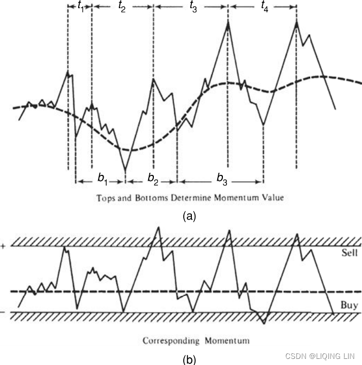 FIGURE 9.6 Relationship of momentum to prices. (a) Tops and bottoms determine momentum value. (b) Corresponding momentum.
 - Momentum and oscillators, however, are more often used to identify abnormal price movements and for timing of entries and exits in conjunction with a longer-term trend. 动量和震荡指标更常用于识别异常价格变动以及结合长期趋势确定进入和退出的时机。
Timing an Entry确定进入的时机
Momentum is a convenient way of identifying good entry points based on small price reversals within a trend that are not large enough to change the direction of the trend. By choosing a much shorter time period for the momentum calculation (for example, 6 days) to work in combination with a longer trend of 30 to 50 days, the momentum indicator will show frequent opportunities within the trend. The short time period for the momentum calculation assures you that there will be an entry opportunity within about 3 days of the entry signal; therefore, it becomes a practical timing tool. This is particularly useful when you view momentum as a countertrend signal, which will be discussed in the next section. Examples of using a momentum as entry timing can also be found in Chapter 19.
Identifying and Fading Price Extremes识别和消退价格极端
An equally popular and more interesting use for momentum focuses on the analysis of relative tops and bottoms. All momentum values are bounded (although somewhat irregularly) in both directions by the maximum move possible during the time interval represented by the span of the momentum. The conditions at the points of high positive and negative momentum are called overbought and oversold, respectively.
A market is
- overbough when it can no longer sustain the strength of the current uptwards trend and a downward price reaction is imminent / ˈɪmɪnənt /即将发生的,临近的;
- an oversold market is ready for an upward move.
- Faster momentum calculations (those using shorter calculation periods) will tend to fluctuate above and below the zero line based on small price changes.
- Longer calculation periods will take on the characteristics of a trend and stay above or below the zero line for the extent of the trend.较长的计算周期将呈现趋势特征,并在趋势范围内保持在零线上方或下方
In Figure 9.7, using S&P futures,
- the 20-day momentum in the center panel stays above zero for most of the period from September 2010 through February 2011.
- The very fast 3-day momentum in the bottom panel consistently penetrates the zero line, although the peaks on the upside are larger than those on the downside.
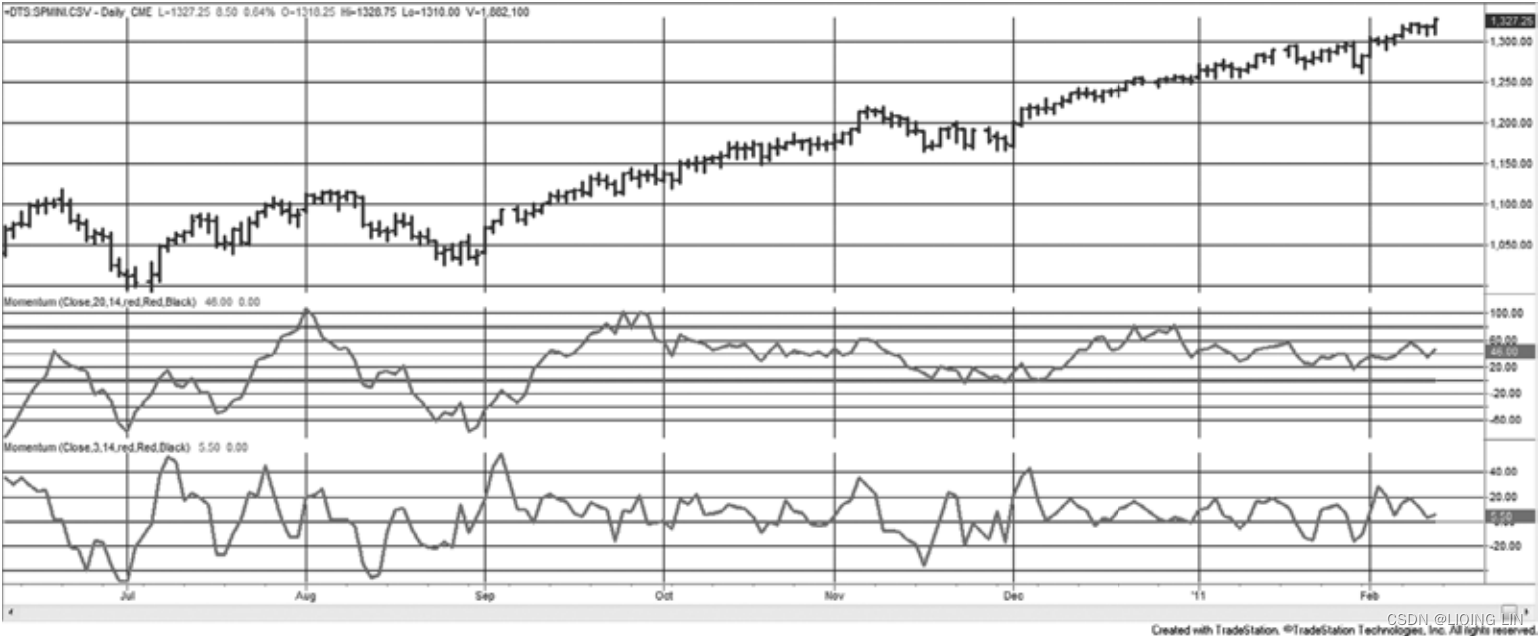 FIGURE 9.7 20-day momentum (center panel) and 3-day momentum (bottom panel) applied to
the S&P, June 2010 through February 2011.
The values on the right scale of the two lower panels in Figure 9.7 show the range of price movement over the 20-day and 3-day periods. The 20-day scale goes from +100 to –60 while the 3-day scale is smaller, about +60 to –40. The 3-day momentum is not 3/20ths of the 20-day momentum(3 天动量不是 20 天动量的 3/20) because volatility does not increase linearly over time. That is, volatility can increase faster in a few days, but over longer periods it has up and down movement that limits the total move in one direction. 波动率在几天内可能会增加得更快,但在更长的时间里,它会上下波动,从而限制一个方向的总波动。
A system can take advantage of the momentum extremes by fading the price movement (selling rallies and buying declines逢高卖出和下跌买入). This is done by drawing two horizontal lines on the momentum chart (as shown in Figure 9.6b) above and below the zero line in such a way that the tops and bottoms of the major moves are isolated. These lines may be selected
- • Visually, so that once the line is penetrated/ ˈpenətreɪtɪd /穿透, prices reverse shortly afterwards.
- • Based on a percentage of the maximum possible momentum value.
- • A multiple of the standard deviation of momentum values. Using two standard deviations would position the lines so that only 5% of all momentum values penetrate above and below the two horizontal lines
When positioning these bands, there is always a trade-off between finding more trading opportunities and entering the market too soon. This can be a complicated choice and is discussed in “System Trade-Offs” in Chapter 22. Once these lines have been drawn, the entry options will be one of the following basic trading rules:
- • Aggressive.
- Enter a new long position when the momentum value penetrates the lower bound;
- enter a new short position when the value penetrates the upper bound.
- • Minor confirmation.
- Enter a new short position on the first day the momentum value turns down after penetrating the upper bound
- (the opposite for longs).
- Enter a new short position on the first day the momentum value turns down after penetrating the upper bound
- • Major confirmation.
- Enter a new short position when the momentum value penetrates the upper bound moving lower
- (the opposite for longs).
- • Timing.
- Enter a new short position after the momentum value has remained above the upper bound for n days
- (the opposite for longs).
To close out a profitable平仓获利的 short or long position, there are the following alternatives (the rules are symmetrical for longs and shorts):
- • Most demanding.
- Close out long positions or cover shorts when the momentum value satisfies the entry condition for a reverse position.当动量值满足反向头寸的入场条件时,平掉多头头寸或回补空头头寸。
- • Moderately demanding.
- Cover a short position when the momentum penetrates the 0 line, minus one standard deviation (or some other target point partway between the zero line and the lower bound).当动量穿透零线,减去一个标准偏差(或零线和下限之间的某个其他目标点)时平仓。
- • Basic exit. Cover a short position when the momentum value becomes 0.
- • Allowing an extended move.
- Cover a short position if the momentum crosses the 0 line moving up after penetrating that line moving down.
The basic exit, removing your trade when the momentum reaches the 0 line, is the benchmark case. It is based on the conservative/kənˈsɜːrvətɪv/保守的 assumption that prices will return to the center of the recent movement (in other words, mean reverting). It is less reasonable to assume that prices will continually move from overbought to oversold and back again. Most statisticians would agree that the mean is the best forecast of future prices, and the 0 momentum value represents the mean. You may try to increase the profits by assuming that the momentum value will penetrate the zero line by a small amount 您可以通过假设动量值会少量穿过零线来尝试增加利润 because there is always some amount of noise. However, if you require a larger penetration of zero to cause an exit, many of the exit opportunities will be lost如果您需要更大的零渗透来导致退出,那么许多退出机会将会丢失 You can be more conservative by exiting somewhat before the zero line is reached, but then you also reduce your average profit.您可以通过在达到零线之前稍微退出来更加保守,但这样您也会降低平均利润。
The same momentum calculations, viewed over a longer time period, show one of the problems with using momentum for timing. Figure 9.8 covers a critical period, from August 2005 through February 2011. Notice that the scale of the momentum values change dramatically from the beginning to the end of the chart.
- This is especially important for the 20-day momentum in the middle panel. For all of 2006, volatility was very low. Had we used momentum as an overbought/oversold indicator, the entry bands would have been at about ±30.
- For the 3-day momentum, it would have been closer to ±15.
- As we saw before, the faster momentum is more symmetric than the slower one. During 2006, there were more selling than buying opportunities(注意 : 多个向下穿过水平线).
 FIGURE 9.8 A longer view of the 20- and 3-day momentum applied to the S&P. The magnitude
of the momentum values change over time.
Volatility increases in 2007. If buy entries were targeted as momentum values of −30 then traders would have held a 120 point loss as momentum dropped to −150. A similar pattern was repeated on the upside for sell signals. It would be necessary to increase the width of the buy and sell bands to ±75 and still hold larger losses waiting for a price reversal. But then comes 2008, and any countertrend entry, buying as prices fall, would have caused a complete loss of equity. However, let’s say that we were able to avoid disaster and the entry-exit bands were at ±100 for the 20-day momentum and ±50 for the 3-day. Volatility finally declines and we get only the occasional entry signal. The bands need to be adjusted back down to a smaller range.
The problem with using momentum for timing is that the scale is unpredictable. Even if we waited for a reversal after penetrating the band there is no assurance that prices will not reverse and go to new extremes. Some risk protection is needed, a way of dynamically adjusting the bands (as discussed in Chapter 8), or a different way of measuring momentum.
Risk Protection
A protective stop-loss order can be used whenever you trade against the current price momentum. A stop-loss is a specific order to exit if the price goes the wrong way (discussed in Chapter 23 but also throughout the book). This is most important with the aggressive entry激进的入场, which advocates selling when the momentum value moves above the upper threshold line, regardless of how fast prices are rising. While the other entry options allow for a logic positioning of a stop-loss其他入场选项允许止损的逻辑定位, the aggressive entry does not. You will simply need to decide, based on historic momentum values, where to limit your risk 您只需要根据历史动量值来决定在何处限制您的风险. With the other entry options, prices are no longer at their extremes于其他入场选项,价格不再处于极端, so that stops may be placed using one of the following techniques:
- • Place a protective stop above or below the most extreme high or low momentum value.在最高或最低动量值上方或下方设置保护性止损
- • Follow a profitable move with a trailing, nonretreating stop based on fixed points or a percentage.遵循基于固定点或百分比的追踪、非撤退止损的获利走势。
- • Establish zones that act as levels of attainment (using horizontal lines of equal spacing), and do not permit reverse penetrations once a new zone is entered.建立作为达到水平的区域(使用等间距的水平线),并且一旦进入新区域就不允许反向渗透
Risk protection must be flexible in the way it deals with volatility. As prices reach higher levels, increased volatility will cause momentum tops and bottoms to widen; with low volatility, prices may not be active enough to penetrate the upper or lower bounds.随着价格达到更高水平,波动性增加将导致动量顶部和底部扩大; 在低波动率的情况下,价格可能不够活跃,无法突破上限或下限。 This is shown in Figure 9.8. Therefore, both the profits and risk of a trade entered at extremes must increase with volatility and higher prices. Stops could be based on a percentage of price or a multiple of volatility进入极端交易的利润和风险都必须随着波动性和更高的价格而增加。 止损可以基于价格的百分比或波动率的倍数。.
The aggressive entry option remains the greatest problem for controlling risk, where a short signal is given when prices are very strong. If an immediate reversal does not occur, large open losses may accrue. To determine the proper stop-loss amount, a computer test was performed using an immediate entry based on penetration of an extreme boundary and with a stop-loss at the close of the day for risk protection. The first results were thought to have outstanding profits and consistency until it was discovered that the computer had done exactly the opposite of what was intended—it bought when the momentum crossed the upper bound and placed a close stop-loss below the entry. It did prove, for a good sampling of futures markets, that high momentum periods continued for enough time to capture small but consistent profi ts. It also showed that the aggressive entry trading rule, anticipating an early reversal, would be a losing strategy. One should never forget that declining momentum does not mean that prices are falling.激进的进场选择仍然是控制风险的最大问题,当价格非常强劲时会发出空头信号。 如果没有立即发生逆转,则可能会累积大量未平仓损失。 为了确定适当的止损金额,我们使用基于突破极端边界的即时入场和在当日收盘时设置止损以保护风险进行了计算机测试。 最初的结果被认为具有出色的利润和一致性,直到发现计算机所做的与预期的完全相反——它在动量越过上限时买入,并在入口下方设置了止损。 它确实证明,对于一个很好的期货市场样本,高动能期持续了足够长的时间来获取小而稳定的利润。 它还表明,预期早期逆转的进取交易规则将是一种失败的策略。 人们永远不应忘记,势头下降并不意味着价格正在下跌。
The Trend Provides Protection
In these examples, momentum is not a strategy itself, but a way of entering a trend trade. When a trend signal first occurs, it is not entered. If the signal was long, then the strategy waits until the 3-day momentum penetrates the lower band. If prices continue lower, then the trend will change from up to down, and the position will be exited. It would not be necessary to have a stop-loss.
Profit Targets for Fading Extreme Moves消退极端走势的利润目标
When using momentum as a mean-reversion strategy, the most reasonable exit for a short entered at an extreme momentum high, or a long position entered at a low, is when the momentum returns to near zero. Prices do not have an obligation to go from extreme lows to extreme highs; however, any extreme can be expected to return to normal, which is where momentum is zero. Returning to zero does not mean that all trades will be profitable. If there has been a strong upwards move that lasted longer than the calculation period of the momentum, then prices will be higher when momentum finally returns to zero. The trend is not your friend if it fights with your mean-reversion position.
The number of profitable trades can be increased by targeting a momentum level that is more conservative than zero. That is, if a long was entered at an extreme low, a sell would be placed 5% or 10% below the zero momentum line, based on the distance between the buying threshold line and zero. Trades that almost return to normal would then be closed out with profits, although the average size of the profi t would be smaller. To increase the size of the profits per trade, you would target the opposite side of the zero momentum line; therefore, if you held a long position, you would wait until the momentum value was greater than zero by 5% or 10% of the range. The success of taking profits early or late depends on the amount of noise in the momentum values as it fluctuates near the zero value. In many cases where extreme prices are followed by a sideways pattern, momentum will fluctuate around zero so that there is ample opportunity to exit the trade at a better price.在许多情况下,极端价格之后是横向形态,动量将在零附近波动,因此有足够的机会以更好的价格退出交易。
High-Momentum Trading
Some professional traders have made a business of trading in the direction of the price move only when momentum exceeds the high threshold level rather than anticipating a change of direction. There is a small window of opportunity when prices are moving fast. They will usually continue at the same, or greater, momentum for a short time, measured usually in minutes or hours, but occasionally a few days. There is a lot of money to be made in a short time—but at great risk if prices reverse direction sooner than expected.
Price patterns have changed. There are many more day traders. When one stock breaks out above a previous high, everyone sees it as an opportunity for profit. Buy orders start to flow, and volume increases. Stocks that are normally ignored can attract large volume when prices make a new high. Traders ride the rising prices for as long as possible, watching to see when volume begins to drop, then they exit. Some may just target a modest profit and get out when that target is reached.
High-momentum trading is a fast game that requires tools that allow you to scan a wide range of stocks. You are looking for one that has made a new high after a long, quiet period寻找经过长期平静期后创下新高的股票. You may also continually sort stocks by the highest momentum values还可以根据最高动量值不断对股票进行排序. You need to stay glued to your screen, enter fast and exit fast您需要紧盯着屏幕,快速进入并快速退出. It is a full-time commitment.
(MACD Trend indicator)Moving Average Convergence/Divergence
 Many of the practical problems of fading prices using momentum are solved with the Moving Average Convergence Divergence (MACD), developed by Gerald Appel. The MACD uses momentum calculated as the difference between two trendlines, produced using exponential smoothing. This momentum value is further smoothed to give a signal line. The most common form of MACD uses the difference between a 12-day and 26-day exponential smoothing. The signal line, used to produce trading recommendations, is a 9-day smoothing of the MACD. The MACD can be created as follows:
- Step 1: Choose the two calculation periods for the trend,
- for example, 20 and 40.
- Convert to smoothing constants(smoothing factors) using 2/(n + 1).
- Step 2: Calculate the slow trendline, EMA40, using the smoothing value 0.0243
 .
. - Step 3: Calculate the fast trendline, EMA20, using the smoothing value 0.0476.

- Step 4: The MACD line, the slower-responding line in the bottom panel of Figure 9.9, is EMA20 – EMA40. When the market is moving up quickly, the fast smoothing will be above the slow, and the difference will be positive. This is done so that the MACD line goes up when prices go up.
- Step 5: The signal line is the 9-day smoothing (using a constant of 0.10) of the MACD line. The signal line is slower than the MACD; therefore, it can be seen in the bottom panel of Figure 9.9 as the lower line when prices are moving higher.t2_Deciphering the Market_ticklabels_sma_ewma_apo_macd_Bollinger_Momentum_statsmodels_adfuller_ARIMA_LIQING LIN的博客-CSDN博客
ema_fast = (close_price - ema_fast) * K_fast + ema_fastclose = goog_data['Close'] num_periods_fast = 20 # time period for the fast EMA K_fast = 2/(num_periods_fast+1) # smoothing factor for fast EMA ema_fast = 0 # initial ema num_periods_slow = 40 # time period for slow EMA K_slow = 2/(num_periods_slow+1) # smoothing factor for slow EMA ema_slow = 0 # initial ema num_periods_macd = 9 # MACD ema time period K_macd = 2/(num_periods_macd+1) # MACD EMA smoothing factor ema_macd= 0 ema_fast_values = [] # we will hold fast EMA values for visualization purposes ema_slow_values = [] # we will hold slow EMA values for visualization purposes macd_values = [] # tract MACD values for visualization purpose # MACD = EMA_fast - EMA_slow macd_signal_values = [] # MACD EMA values tracker # MACD_signal = EMA_MACD macd_histogram_values = [] # MACD = MACD - MACD_signal for close_price in close: if ema_fast == 0: # first observation ema_fast = close_price ema_slow = close_price else: ema_fast = (close_price - ema_fast) * K_fast + ema_fast ema_slow = (close_price - ema_slow) * K_slow + ema_slow ema_fast_values.append( ema_fast ) ema_slow_values.append( ema_slow ) macd = ema_fast - ema_slow # MACD is fast_MA - slow_EMA # apo_values if ema_macd == 0 : ema_macd = macd else: ema_macd = (macd-ema_macd) * K_macd + ema_macd # signal is EMA of MACD values macd_values.append( macd ) macd_signal_values.append( ema_macd ) macd_histogram_values.append( macd-ema_macd )
ema_slow = (close_price - ema_slow) * K_slow + ema_slow
adjust=False

adjust=True ==> Expanding out EMA_old...

等式的上方是对当前价格到最初价格的加权求和,用的加权因子是
等式的下方是对所有加权因子的求和(可用等比例求和公式)
等比例求和公式推导
 and
and (公比
(公比 )
)

 ==>
==>
mpf11_3_status_plotly Align dual Yaxis_animation_button_MFI_Williams %Rsi_AO Co_VWAP_MAcd_BollingerB_LIQING LIN的博客-CSDN博客
def get_macd( df, MACD_EMA_SHORT=12, MACD_EMA_LONG=26, MACD_EMA_SIGNAL=9 ):
    """ Moving Average Convergence Divergence
    This function will initialize all following columns.
    MACD Line (macd): (12-day EMA - 26-day EMA)
    Signal Line (macds): 9-day EMA of MACD Line
    MACD Histogram (macdh): MACD Line - Signal Line
    :param df: data
    :return: None
    """
    close = df['Close']

    fast = close.ewm(ignore_na=False,
                     span=MACD_EMA_SHORT,# span:window size ==> a=2/(span+1) : decay or smoothing factor
                     min_periods=0, # Minimum number of observations in window required to have a value
                     adjust=True    # the EW function is calculated using weights
                    ).mean()
    slow = close.ewm(ignore_na=False,
                     span=MACD_EMA_LONG,# span:window size ==> a=2/(span+1) : decay or smoothing factor
                     min_periods=0, # Minimum number of observations in window required to have a value
                     adjust=True    # the EW function is calculated using weights
                    ).mean()
    df['macd'] = fast - slow
    # Signal Line (macds): 9-day EMA of MACD Line
    df['macds_{}'.format(MACD_EMA_SIGNAL)] = df['macd'].ewm(ignore_na=False,
                                                           span=MACD_EMA_SIGNAL,# span:window size ==> a=2/(span+1) : decay or smoothing factor
                                                           min_periods=0, # Minimum number of observations in window required to have a value
                                                           adjust=True    # the EW function is calculated using weights
                                                          ).mean()
    df['macdh_{}_{}'.format(MACD_EMA_SHORT, MACD_EMA_LONG)] = (df['macd'] - df['macds_{}'.format(MACD_EMA_SIGNAL)]) # MACD Histogram (macdh): MACD Line - Signal Line

    return df
The 20- and 40-day momentum lines(NOTE The term momentum is very flexible. It is common for it to refer to the difference between today’s price and a corresponding moving average value: and
), corresponding to the MACD line and the histogram, are shown in the center panel of Figure 9.9.
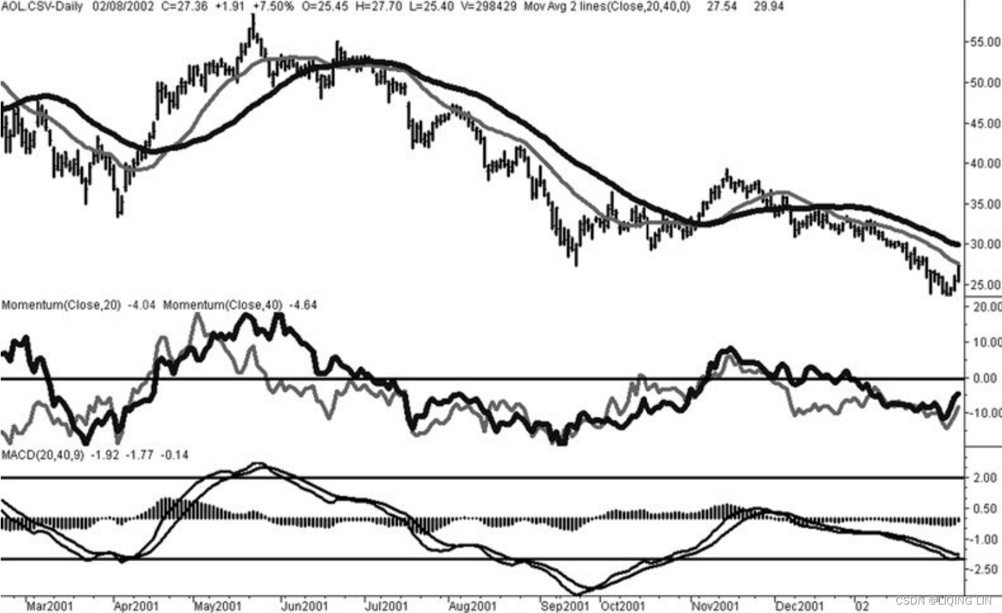 FIGURE 9.9 MACD for AOL. The MACD line is the faster of the two trendlines in the bottom panel; the signal line is the slower. The histogram is created by subtracting the slower signal line
from the MACD line.
It is clear that the MACD process smoothes these values significantly; therefore, it makes trading signals easier to see.
Trading the MACD
The most common use of the MACD is as a trend indicator. For this purpose, only the MACD and signal lines are used in the following way:
- Buy when the MACD line (faster) crosses upwards through the signal line (slower).
- Sell when the MACD line crosses from above to below the signal line.
In the bottom panel of Figure 9.9, the buy signals that occur right after an extreme low in April and October of 2001 generated large gains. Unfortunately, there were many other crossings that generated losses; therefore, it is necessary to select which trades to enter. To accomplish that, the MACD uses thresholds similar to those shown for momentum, but in the opposite way. The MACD must first penetrate the lower band; then it must signal a new uptrend before a long position can be entered. In this way, it removes some of the whipsaws that might occur in a sideways market. Threshold levels were established by observing the historically high and low momentum values, shown as horizontal lines at the +2.00 and −2.00 levels in Figure 9.9. Sell signals would have been taken only after the MACD value had been above +2.00, and buy signals only when the MACD value had fallen below −2.00. The trading signals that satisfy these conditions are the buy signal in April, a sell a in May, and a buy a in October. However, fitting the threshold lines make them unreliable values for trading但是,拟合阈值线会使它们成为不可靠的交易值. One solution can be found in “An RSI Version of MACD” in the next section.
Appel has written extensively on the MACD, and many variations can be found in his book, Technical Analysis( Gerald Appel, Technical Analysis, Power Tools for Active Investors (Upper Saddle River, NJ: FT Prentice Hall, 2005) ). Many of the examples are interpretive, similar to the way we look at chart patterns. Appel also preferred using trends of 19 and 39 days for the NASDAQ composite. An equally important use of MACD is for divergence signals. Bearish divergence occurs when prices are rising but the MACD values are falling. Because this technique applies to many indicators in addition to the MACD, it is covered in detail in the section “Momentum Divergence” toward the end of this chapter.
Interpretation
- The Moving Average Convergence/Divergence (MACD, or MAC-D) line is calculated by subtracting the 26-period exponential moving average (EMA) from the 12-period EMA. The signal line is a 9-period EMA of the MACD line.
- MACD is best used with daily periods, where the traditional settings of 26/12/9 days is the norm.
- MACD triggers technical signals when the MACD line crosses above the signal line (to buy) or falls below it (to sell).
- MACD can help gauge/ ɡeɪdʒ / whether a security is overbought or oversold, alerting traders to the strength of a directional move, and warning of a potential price reversal.
MACD 可以帮助衡量证券是超买还是超卖,提醒交易者定向移动的强度,并警告潜在的价格反转。 - MACD can also alert investors to bullish/bearish divergences (e.g., when a new high in price is not confirmed by a new high in MACD, and vice versa), suggesting a potential failure and reversal.
MACD 还可以提醒投资者注意看涨/看跌背离(例如,当 MACD 的新高未确认价格的新高时,反之亦然),表明潜在的失败和逆转。 - After a signal line crossover, it is recommended to wait for three or four days to confirm that it is not a false move.
信号线交叉后,建议等待三四天,确认不是假动作。
As its name implies, the MACD is all about the convergence and divergence of the two exponential moving averages. Convergence occurs when the moving averages move towards each other. Divergence occurs when the moving averages move away from each other. The shorter moving average (12-day) is faster and responsible for most MACD movements. The longer moving average (26-day) is slower and less reactive to price changes in the underlying security.
The MACD line oscillates above and below the zero line, which is also known as the centerline. These crossovers signal that the 12-day EMA has crossed the 26-day EMA. The direction, of course, depends on the direction of the moving average cross.
- Positive MACD indicates that the 12-day EMA is above the 26-day EMA. Positive values increase as the shorter EMA diverges further from the longer EMA. This means upside momentum is increasing.
- Negative MACD values indicate that the 12-day EMA is below the 26-day EMA. Negative values increase as the shorter EMA diverges further below the longer EMA. This means downside momentum is increasing.
 In the example above,
- the yellow area shows the MACD line in negative territory as the 12-day EMA trades below the 26-day EMA. The initial cross occurred at the end of September (black arrow) and the MACD moved further into negative territory as the 12-day EMA diverged further from the 26-day EMA.
- The orange area highlights a period of positive MACD values, which is when the 12-day EMA was above the 26-day EMA.
Notice that the MACD line remained below 1 during this period (red dotted line). This means the distance between the 12-day EMA and 26-day EMA was less than 1 point, which is not a big difference. 请注意,MACD 线在此期间保持在 1 以下(红色虚线)。 这意味着 12 天 EMA 和 26 天 EMA 之间的距离小于 1 点,相差不大。
Signal Line Crossovers
信号线交叉是最常见的 MACD 信号。 信号线是 MACD 线的 9 天 EMA。 作为指标的移动平均线,它落后于 MACD 并且更容易发现 MACD 转向。
- 当 MACD 向上并穿过信号线时,出现bullish crossover。
- 当 MACD 向下并穿过信号线下方时,出现bearish crossover。
- 交叉可以持续几天或几周,具体取决于移动的强度。
当交叉符合流行趋势时,它们更可靠。 如果 MACD 在长期上升趋势中经过短暂的下行修正后上穿其信号线,则有资格确认看涨并可能延续上升趋势。 
如果 MACD 在长期下降趋势中短暂走高后下穿信号线,交易员会认为这是看跌确认。
Due diligence尽职调查/ ˈdɪlɪdʒəns / is required before relying on these common signals. Signal line crossovers at positive or negative extremes should be viewed with caution. Even though the MACD does not have upper and lower limits, chartists can estimate historical extremes with a simple visual assessment. It takes a strong move in the underlying security to push momentum to an extreme. Even though the move may continue, momentum is likely to slow and this will usually produce a signal line crossover at the extremities. Volatility in the underlying security can also increase the number of crossovers.
MACD 通常以直方图(见下图)显示,该直方图描绘了 MACD 与其信号线之间的距离。 如果 MACD 高于信号线,则直方图将高于 MACD 的基线或零线。 如果 MACD 低于其信号线,则直方图将低于 MACD 的基线。 交易者使用 MACD 的柱状图来确定何时看涨或看跌势头高——以及可能超买/超卖。
 The chart shows IBM with its 12-day EMA (green), 26-day EMA (red) and the 12,26,9 MACD in the indicator window. There were eight signal line crossovers in six months: four up and four down. There were some good signals and some bad signals. The yellow area highlights a period when the MACD line surged above 2 to reach a positive extreme. There were two bearish signal line crossovers
![]() in April and May, but IBM continued trending higher. Even though upward momentum slowed after the surge, it was still stronger than downside momentum in April-May. The third bearish signal line crossover
in April and May, but IBM continued trending higher. Even though upward momentum slowed after the surge, it was still stronger than downside momentum in April-May. The third bearish signal line crossover![]() in May resulted in a good signal.
in May resulted in a good signal.
Centerline Crossovers
Centerline crossovers are the next most common MACD signals.
- A bullish centerline crossover occurs when the MACD line moves above the zero line to turn positive. This happens when the 12-day EMA of the underlying security moves above the 26-day EMA.
- A bearish centerline crossover occurs when the MACD line moves below the zero line to turn negative. This happens when the 12-day EMA moves below the 26-day EMA.
- Centerline crossovers can last a few days or a few months, depending on the strength of the trend.
- The MACD will remain positive as long as there is a sustained uptrend.
- The MACD will remain negative when there is a sustained downtrend.
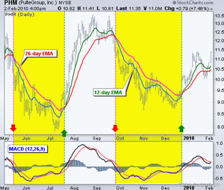 The chart shows Pulte Homes (PHM) with at least four centerline crosses in nine months. The resulting signals worked well because strong trends emerged with these centerline crossovers.
The chart of Cummins Inc (CMI) with seven centerline crossovers in five months. In contrast to Pulte Homes, these signals would have resulted in numerous whipsaws because strong trends did not materialize after the crossovers.与 Pulte Homes 相比,这些信号会导致大量洗盘,因为在交叉之后没有出现强劲趋势。
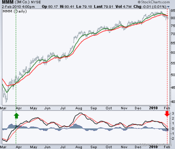 The chart shows 3M (MMM) with a bullish centerline crossover in late March 2009 and a bearish centerline crossover in early February 2010. This signal lasted 10 months. In other words, the 12-day EMA was above the 26-day EMA for 10 months. This was one strong trend.
Divergences
Divergences form when the MACD diverges from the price action of the underlying security. A bullish divergence forms when a security records a lower low and the MACD forms a higher low. The lower low in the security affirms the current downtrend, but the higher low in the MACD shows less downside momentum. Despite decreasing, downside momentum is still outpacing upside momentum as long as the MACD remains in negative territory尽管下降,但只要 MACD 仍处于负区域,下行势头仍超过上行势头. Slowing downside momentum can sometimes foreshadow a trend reversal or a sizable rally下行势头放缓有时预示着趋势逆转或大幅反弹.
 The chart shows Google (GOOG) with a bullish divergence in October-November 2008.
- First, notice that we are using closing prices to identify the divergence. The MACD's moving averages are based on closing prices and we should consider closing prices in the security as well.
- Second, notice that there were clear reaction lows (troughs) as both Google and its MACD line bounced in October and late November.
- Third, notice that the MACD formed a higher low as Google formed a lower low in November. The MACD turned up with a bullish divergence and the subsequent signal line crossover in early December. Google confirmed a reversal with a resistance breakout.
A bearish divergence forms when a security records a higher high and the MACD line forms a lower high. The higher high in the security is normal for an uptrend, but the lower high in the MACD shows less upside momentum. Even though upside momentum may be less, upside momentum is still outpacing downside momentum as long as the MACD is positive.尽管上行势头可能减弱,但只要 MACD 为正,上行势头仍超过下行势头。 Waning upward momentum can sometimes foreshadow a trend reversal or sizable decline. 上升势头减弱有时预示着趋势逆转或大幅下跌。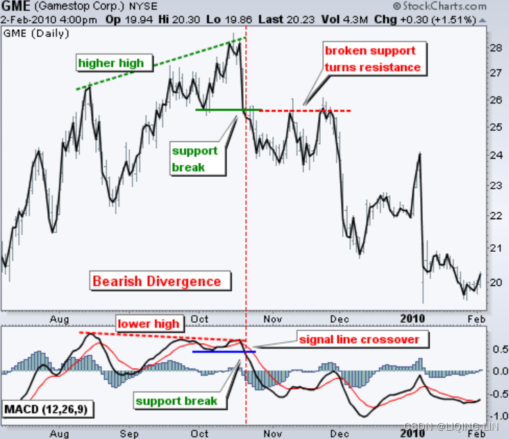
we see Gamestop (GME) with a large bearish divergence from August to October. The stock forged a higher high above 28, but the MACD line fell short of its prior high and formed a lower high. The subsequent signal line crossover and support break in the MACD were bearish. On the price chart, notice how broken support turned into resistance on the throwback bounce in November (red dotted line). This throwback provided a second chance to sell or sell short.
Divergences should be taken with caution. Bearish divergences are commonplace in a strong uptrend, while bullish divergences occur often in a strong downtrend. Yes, you read that right. Uptrends often start with a strong advance that produces a surge in upside momentum (MACD). Even though the uptrend continues, it continues at a slower pace that causes the MACD to decline from its highs. Upside momentum may not be as strong, but it will continue to outpace downside momentum as long as the MACD line is above zero.上行势头可能不那么强劲,但只要 MACD 线高于零,上行势头就会继续超过下行势头 The opposite occurs at the beginning of a strong downtrend相反的情况发生在强劲下降趋势的开始. 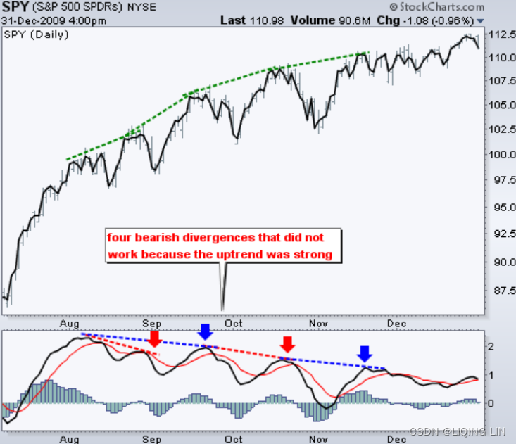 The chart shows the S&P 500 ETF (SPY) with four bearish divergences from August to November 2009. Despite less upside momentum, the ETF continued higher because the uptrend was strong. Notice how SPY continued its series of higher highs and higher lows. Remember, upside momentum is stronger than downside momentum as long as the MACD is positive.请记住,只要 MACD 为正,上行势头就强于下行势头 The MACD (momentum) may have been less positive (strong) as the advance extended, but it was still largely positive.随着上涨的扩大,MACD(动量)可能不那么积极(强劲),但它在很大程度上仍然是积极的。
MACD vs. Relative Strength
相对强弱指数 (RSI) 旨在表明市场相对于近期价格水平是否被视为超买或超卖。 RSI 是一个震荡指标,计算给定时间段内的平均价格收益和损失。 默认时间段为 14 个周期,值介于 0 到 100 之间。读数高于 70 表明超买情况,而低于 30 的读数被认为超卖,两者都可能表明顶部正在形成,反之亦然(底部正在形成 ).
然而,MACD 线并没有像 RSI 和其他振荡器研究那样具体的超买/超卖水平。 相反,它们是在相对的基础上发挥作用的。 也就是说,与手头证券的先前价格变动相比,投资者或交易者应关注 MACD/信号线的水平和方向,如下所示。 MACD measures the relationship between two EMAs, while the RSI measures price change in relation to recent price highs and lows. These two indicators are often used together to give analysts a more complete technical picture of a market.
这些指标都衡量市场的动能,但由于它们衡量的因素不同,因此有时会给出相反的指示。 例如,RSI 可能会在一段时间内显示高于 70(超买)的读数,表明市场相对于近期价格过度扩张至买方,而 MACD 表明市场的购买势头仍在增加。 任一指标都可能通过显示与价格的背离来预示即将发生的趋势变化(价格继续走高而指标转低,反之亦然)。
Limitations of MACD and Confirmation
移动平均线背离的主要问题之一是它通常可以发出可能的逆转信号,但实际上并没有发生逆转——它会产生误报。 另一个问题是背离并不能预测所有的逆转。 换句话说,它预测了太多没有发生的反转,并且没有足够的实际价格反转。
这表明应通过趋势跟踪指标寻求确认,例如方向运动指数 (DMI) 系统及其关键组成部分平均方向指数 (ADX)。
Plus Directional Movement (+DM)
- Use +DM when current high - previous high > previous low - current low.
if UpMove > DownMove and UpMove > 0,
then +DM = UpMove,
else
+DM = 0 #A negative value would simply be entered as zero
Minus Directional Movement (-DM)
- Use -DM when previous low - current low > current high - previous high.
if DownMove > UpMove and DownMove > 0,
then -DM = DownMove,
else
-DM = 0 #A negative value would simply be entered as zero
Smooth the 14-period averages of +DM, -DM, and TR—the TR formula is below. Insert the -DM and +DM values to calculate the smoothed averages of those.
TR is the greater of the current high - current low, current high - previous close, or current low - previous close.![]()
- First TR14 = sum of first 14 TR
- Second TR14 = First TR14 - (First TR14 /14) + Current TR1
- Subsequent Values = Prior TR14 - (Prior TR14 /14) + Current TR1


Directional Movement Index :
Average Directional Index
- First ADX14 = 14 period Average of DX
- Second ADX14 = ((First ADX14 x 13) + Current DX Value)/14
- Subsequent ADX14 = ((Prior ADX14 x 13) + Current DX Value)/14
import numpy as np
import pandas as pd

def get_adx(df, window=14):
        """ get the default setting for Average Directional Index(Average Directional Movement Index)
        """
        # +DM = current high - previous high
        # -DM = previous low - current low
        dm = pd.DataFrame( dict(enumerate([ df['High'] - df['High'].shift(1, fill_value=np.nan),
                                            df['Low'].shift(1,fill_value=np.nan) - df['Low']
                                          ])
                               )
                         )
        #                             +DM>0      +DM > -DM
        df['+dm'] = dm.apply( lambda m: max(m[0],0) if m[0]>m[1] else 0, axis=1)
        #                             -DM>0      -DM > +DM
        df['-dm'] = dm.apply( lambda m: max(m[1],0) if m[1]>m[0] else 0, axis=1)

#         df['tr']=pd.DataFrame(dict(enumerate([df['High']-df['Low'],
#                                               abs( df['High']-df['Close'].shift(1) ),
#                                               abs( df['Low']-df['Close'].shift(1) )
#                                              ])
#                                   )
#                              ).apply(max,axis=1)
# OR
        df['TrueLow'] = pd.DataFrame(dict(enumerate([ df['Low'],
                                                  df['Close'].shift(1),
                                                ])
                                    )
                               ).apply( min,axis=1 )
        df['TrueHigh'] = pd.DataFrame(dict(enumerate([ df['High'],
                                                   df['Close'].shift(1),
                                                 ])
                                    )
                               ).apply( max,axis=1 )
        df.loc[df.index[0],[ 'TrueLow', 'TrueHigh'] ]=np.nan # since df['Close'].shift(1)
        # true range
        df['tr'] = df['TrueHigh'] - df['TrueLow']
######
        df.loc[df.index[0],['+dm', '-dm', 'tr']]=np.nan # for window
        def smooth(col):

            sm=col.rolling(window).sum()
            for i in list( range( window+1,len(col) ) ):
                #sm.iloc[i]=sm.iloc[i-1]-(1.0*sm.iloc[i-1]/window)+col.iloc[i]
                sm.iloc[i]=col.iloc[i] + (1.0-1.0/window)*sm.iloc[i-1]

            return sm

        def smooth2(col):
            sm=col.rolling(window).mean()
            for i in list( range( window*2,len(col) ) ):
                #sm.iloc[i]=((sm.iloc[i-1]*(window-1))+col[i])/window
                sm.iloc[i]=(1.0/window)*col.iloc[i] + (1-1.0/window)*sm.iloc[i-1]

            return sm

        df['smoothed +dm'] = df.loc[:,['+dm']].apply(smooth)
        df['smoothed -dm'] = df.loc[:,['-dm']].apply(smooth)
        df['smoothed tr'] = df.loc[:,['tr']].apply(smooth)

        df['+di_{}'.format(window)] = 100.0 * df['smoothed +dm'] / df['smoothed tr']
        df['-di_{}'.format(window)] = 100.0 * df['smoothed -dm'] / df['smoothed tr']

        df['di_{}_diff'.format(window)]=(df['+di_{}'.format(window)] - df['-di_{}'.format(window)])

        df['dx_{}'.format(window)] = 100.0 *abs( df['di_{}_diff'.format(window)] ) /\
                                            ( df['+di_{}'.format(window)] + df['-di_{}'.format(window)] )

        df['adx_{}'.format(window)] = df.loc[:,['dx_{}'.format(window)]].apply(smooth2)

        df.drop(columns=['smoothed +dm', 'smoothed -dm', 'smoothed tr',
                         '+dm', '-dm', 'tr',
                         'dx_{}'.format(window)
                         ],
                inplace=True
               )
        return df

qqq = pd.read_excel('adx.xlsx',
                    sheet_name='adx',
                    header=1,
                    index_col=1
                   )

qqq=get_adx(qqq.loc['2009-02-11':'2009-03-25', ['High','Low','Close']],)

qqq
ADX 旨在指示趋势是否存在,读数高于 25 表示趋势存在(任一方向),读数低于 20 表示没有趋势存在。https://blog.csdn.net/Linli522362242/article/details/129849171
遵循 MACD 交叉和背离的投资者在根据 MACD 信号进行交易之前应仔细检查 ADX。 例如,虽然 MACD 可能显示看跌背离,但检查 ADX 可能会告诉您走高趋势已经到位——在这种情况下,您会避开看跌 MACD 交易信号并等待市场在接下来的时间里如何发展 几天。
另一方面,如果 MACD 显示看跌交叉,而 ADX 处于非趋势区域 (<25) 并且可能已经见顶并自行反转,那么您可能有充分的理由进行看跌交易。
此外,当资产价格在盘整中横向移动时,例如在趋势之后的范围或三角形模式中,经常会出现假阳性背离。 价格势头放缓(横向移动或缓慢趋势移动)将导致 MACD 脱离其先前的极值并趋向于零线,即使没有真正的反转也是如此。 同样,在行动之前仔细检查 ADX 以及趋势是否到位。
Conclusion
The MACD indicator is special because it brings together momentum and trend in one indicator. This unique blend of trend and momentum can be applied to daily, weekly or monthly charts. The standard setting for MACD is the difference between the 12- and 26-period EMAs. Chartists looking for more sensitivity may try a shorter short-term moving average and a longer long-term moving average. MACD(5,35,5) is more sensitive than MACD(12,26,9) and might be better suited for weekly charts. Chartists looking for less sensitivity may consider lengthening the moving averages. A less sensitive MACD will still oscillate above/below zero, but the centerline crossovers and signal line crossovers will be less frequent.不太敏感的 MACD 仍将在零上方/下方振荡,但中线交叉和信号线交叉的频率会降低。
MACD 不是特别适合识别超买和超卖水平。 尽管可以识别历史上的超买或超卖水平,MACD 没有任何上限或下限来约束其走势。 在剧烈波动期间,MACD 可能会继续过度扩张,超出其历史极值。
Finally, remember that the MACD line is calculated using the actual difference between two moving averages. This means MACD values are dependent on the price of the underlying security. The MACD values for a $20 stocks may range from -1.5 to 1.5, while the MACD values for a $100 may range from -10 to +10. It is not possible to compare MACD values for a group of securities with varying prices. If you want to compare momentum readings, you should use the Percentage Price Oscillator (PPO), instead of the MACD.不可能比较一组价格不同的证券的 MACD 值。 如果您想比较动量读数,您应该使用百分比价格震荡指标 (PPO),而不是 MACD。
Divergence Index
Standard deviation, which will be referred to as STDEV, is a basic measure of price volatility that is used in combination with a lot of other technical analysis indicators to improve them. We'll explore that in greater detail in this section.
Standard deviation is a standard measure that is computed by measuring the squared deviation of individual prices from the mean price, and then finding the average of all those squared deviation values. This value is known as variance, and the standard deviation is obtained by taking the square root of the variance. Larger STDEVs are
- a mark of more volatile markets or
- larger expected price moves,
- so trading strategies need to factor that increased volatility into risk estimates and other trading behavior.因此,交易策略需要将增加的波动性纳入风险估计和其他交易行为中。
To compute standard deviation, first we compute the variance: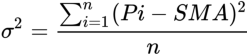
Then, standard deviation is simply the square root of the variance:
SMA : Simple moving average over n time periods.t2_Deciphering the Market_ticklabels_sma_ewma_apo_macd_Bollinger_Momentum_statsmodels_adfuller_ARIMA_LIQING LIN的博客-CSDN博客
A method similar to MACD but one that uses an interesting combination of generalized techniques is the divergence index, the volatility-adjusted difference between two moving averages, for example, 10 and 40 days. Using general notation:
- 1.
= 40-day average of the most recent prices
- 2.
= 10-day average of the most recent prices
- 3.
Then the divergence index (DI),
The standard deviation of the price differences, taken over the slow period of 40, volatility-adjusts the results. The trading rules require a band around zero to trigger entries.
where factor = 1.0. By using the standard deviation of DI, the band also adjusts to changes in volatility波段还可以根据波动率的变化进行调整. In Figure 9.10 the index in the lower panel has high peaks followed by periods of low or varying volatility. The standard deviation allows the bands to widen or narrow according to the pattern of fluctuations标准偏差允许波段根据波动模式加宽或变窄. This example used the slow period for the standard deviation; however, the fast period would have caused more rapid changes to the band这个例子使用标准差的慢周期; 但是,快速周期会导致波段发生更快速的变化。 FIGURE 9.10 Divergence index applied to S&P futures..
The trading rules are
- Buy when the DI moves below the lower band while in an uptrend
- Sell when the DI moves above the upper band while in a downtrend
- Exit longs and shorts when the DI crosses zero
Figure 9.10 shows the DI and the upper and lower bands in the bottom panel. The top panel shows the trading signals for the S&P 500 futures contract.
Oscillator
Because the representation of momentum is that of a line fluctuating above and below a zero value, it has often been termed an oscillator. Even though it does oscillate, the use of this word is confusing. In this presentation, the term oscillator will be restricted to a specific form of momentum that is normalized and expressed in terms of values that are limited to the ranges between +1 and –1 (or +100 to –100), +1 and 0, or +100 and 0 (as in a percent).
To transform a standard momentum calculation into the normalized form with a maximum value of +1 and a minimum value of −1, divide the momentum calculation by its range over the same rolling time period. This allows the oscillator to self-adjust to changes in price or volatility.
For example,
- in April 2006, Amazon was trading at about $34. During a 10-day period it had a high of $35.31 and a low of $31.52, a range of $3.79=35.31-31.52.
- During 10 days in February 2011, Amazon had a high of $191.40 and a low of $174.77, a range of $16.63=191.40-174.77.
- Therefore, a price move of $2 in 2006 would be the same as a move of $8.77 in 2011. By dividing $2 by $3.79 or $8.77 by $16.63 we get 0.52 in both cases.
- Hence, normalization, which is the basis for most momentum indicators, can be an excellent way to self-adjust to price changes.
The following sections show how a number of useful oscillators are calculated. In each case, the purpose is to have the indicator post high values when prices are at a peak and low values when they are in a valley. To be most useful, prices should reverse direction soon after the oscillator records values near its extremes.
(RSI-Momentum indicator)Relative Strength Index
One of the most popular indicators for showing overbought and oversold conditions is the Relative Strength Inde(RSI) developed by Welles Wilder. It provides added value to the concept of momentum by scaling all values between 0 and 100. It is more stable than momentum because it uses all the values in the calculation period rather than just the first and last. It is a simple measurement that expresses the relative strength of the current price movement as increasing from 0 to 100. It is calculated as and
The very first calculations for average gain(Average price change on up days) and average loss(Average price change on down days) are simple 14-period averages:
- First Average Gain = Sum of Gains over the past 14 periods / 14.
- First Average Loss = Sum of Losses over the past 14 periods / 14
The second, and subsequent, calculations are based on the prior averages and the current gain loss:
- Average Gain = [(previous Average Gain) x 13 + current Gain] / 14.
- Average Loss = [(previous Average Loss) x 13 + current Loss] / 14
- at least 250 data points prior to the starting date of any chart
import numpy as np
import pandas as pd

def get_rsi(df, columnName='Adj Close',window=14):
    # https://pandas.pydata.org/docs/reference/api/pandas.Series.diff.html
    # Series.diff(default periods=1) # periods=1 : diff = current row - 1st previous row
    #                                # periods=3 : diff = current row - 3rd previous row
    #                                # periods=-1 : diff = current row - 1st following row
    df['Up Move'] = df[columnName].diff().apply(lambda diff: diff if diff>0 else 0)
    df['Down Move'] = df[columnName].diff().apply(lambda diff: -diff if diff<0 else 0)

    df['Average Up'] = np.nan
    df['Average Down'] = np.nan
    # Calculate initial Average Up & Down, RS and RSI
    # First Average Gain (Average price change on up days)
    df['Average Up'].iloc[window] = df['Up Move'].iloc[1:window+1].mean()     # 1 since df['Up Move'][0] is NaN  <== diff()

    # First Average Loss (Average price change on down days)
    df['Average Down'].iloc[window] = df['Down Move'].iloc[1:window+1].mean() # 1 since df['Down Move'][0] is NaN <== diff()


    # Relative Strength
    df['rs_{}'.format(window)] = np.nan
    # Relative Strength Index
    df['rsi_{}'.format(window)] = np.nan

    df['rs_{}'.format(window)].iloc[window] = df['Average Up'].iloc[window] / df['Average Down'].iloc[window]
    df['rsi_{}'.format(window)].iloc[window] = 100 - ( 100/(1+df['rs_{}'.format(window)].iloc[window]) )


    # Calculate rest of Average Up, Average Down, RS, RSI
    for row_index in range( window+1, len(df) ):

        df['Average Up'].iloc[row_index] = (df['Average Up'].iloc[row_index-1]*(window-1) +\
                                            df['Up Move'].iloc[row_index]
                                           )/window
        df['Average Down'].iloc[row_index] = (df['Average Down'].iloc[row_index-1]*(window-1) +\
                                              df['Down Move'].iloc[row_index]
                                             )/window
        df['rs_{}'.format(window)].iloc[row_index] = df['Average Up'].iloc[row_index] / df['Average Down'].iloc[row_index]
        df['rsi_{}'.format(window)].iloc[row_index] = 100 - (100/(1+df['rs_{}'.format(window)].iloc[row_index]))

    df.drop(columns=['Up Move','Down Move',
                     'Average Up','Average Down',
                     'rs_{}'.format(window)
                    ],
            inplace=True
           )
    return df
All price changes are treated as positive numbers. The daily calculation of the RSI becomes a matter of simple arithmetic. Wilder has favored the use of 14 days because it represents one-half of a natural cycle, in this case, 1 month. He has set the significant threshold levels for the RSI at 30 and 70.
-
Penetration of the lower level is indicative of an imminent upturn and
-
penetration of the upper level, a pending downturn.
-
A chart of an RSI is shown along with a comparable momentum and stochastic indicator in the next section, Figure 9.15.
-
 FIGURE 9.11 RSI top formation.
Use of the RSI alone to generate trading signals often requires interpretation similar to standard chart analysis. Lines are drawn across the tops of the RSI values to indicate a downtrend. A head-and-shoulders formation can be used as the primary confirmation of a change in direction. Wilder himself used the RSI top and bottom formations shown in Figure 9.11. A break of the reaction bottom between the declining tops is a sell signal. In addition, the failure swing, or divergence (discussed later in this chapter), denotes an unsuccessful test of a recent high or low RSI value失败摆动或背离(在本章后面讨论)表示对最近高或低 RSI 值的测试不成功。.
Wilder created other popular indicators. One of these is a momentum calculation called the Average Directional Movement (ADX). The ADX is a byproduct副产品 of the Directional Movement and is discussed in Chapter 23. All of these indicators are actively used by traders.
Modifying the RSI
An obvious objection反对的理由 to the RSI might be the selection of a 14-day half-cycle. Maximum divergence is achieved by using a moving average that is some fraction of the length of the dominant cycle, but 14 days may not be that value. If a 14-day calculation period is too short, then the RSI would remain outside the 70-30 zones for extended periods rather than signaling an immediate turn. In practical terms, a 14-day RSI means that a sustained move in one direction that lasts for more than 14 days will produce a very high RSI value. If prices continue higher for more than 14 days, then the RSI, as with other oscillators, will go sideways. The idea is to pick the calculation period for which there are very few larger sustained moves, and 14 may be that value. If more frequent overbought and over-sold conditions are needed, then the period could be lowered to 10. At the same time, the zones could be increased to 80-20. Some combination of calculation period and zone will usually give the frequency of trades that is needed.对 RSI 的一个明显反对意见可能是选择 14 天半周期。 最大背离是通过使用占主导周期长度的一小部分的移动平均线来实现的,但 14 天可能不是那个值。 如果 14 天的计算周期太短,则 RSI 将长时间保持在 70-30 区域之外,而不是立即转向的信号。 实际上,14 天 RSI 意味着朝一个方向持续移动超过 14 天将产生非常高的 RSI 值。 如果价格持续走高超过 14 天,则 RSI 与其他震荡指标一样将横盘整理。 这个想法是选择几乎没有较大的持续移动的计算周期,14 可能是那个值。 如果需要更频繁的超买和超卖条件,那么周期可以降低到 10。同时,区域可以增加到 80-20。 计算周期和区域的某种组合通常会给出所需的交易频率。
A study by Aan(Peter W. Aan, “How RSI Behaves,”Futures (January 1985).) on the distribution of the 14-day RSI showed that the average RSI top and bottom value consistently grouped near 72 and 32, respectively. Therefore, 50% of all RSI values fall between 72 and 32, which can be interpreted as normally distributed, and equivalent to about 0.675 standard deviations. This would suggest that the 70-30 levels proposed by Wilder are too close together to act as selective overbought/oversold values, but should be moved farther apart. The equivalent of 1.5 standard deviations is a comfortable trade-off between frequency of trades and risk. It is generally safer to err on the side of less risk. If there are too many trades being generated by the RSI, a combination of a longer interval and higher confi dence bands will be an improvement.通常在风险较小的情况下犯错更安全。 如果 RSI 产生的交易太多,则结合使用更长的间隔和更高的置信区间将是一种改进。
Further Smoothing with N-Day Ups and Downs(N日涨跌进一步平滑)
Instead of increasing the number of days in the RSI calculation period, a smoother indicator can be found by increasing the period over which each of the up and down values are determined. 与其增加 RSI 计算周期中的天数,不如通过增加确定每个上升值和下降值的周期来找到更平滑的指标。The original RSI method uses 14 individual days, where an up day is a day in which the price change was positive. Instead, we can replace each 1-day change with a 2-day change, or an n-day change. If we use 2-day changes, then a total of 28 days will be needed, so that each 2-day period does not overlap another; there will be 14 sets of two days each. Using 14 sets of 2 will give a smoother indicator than using 28 single-day changes.
RSI Countertrend Trading
Momentum indicators are used for timing and countertrend trading. Normally, it is the absolute overbought or oversold level that is the trigger for a trade. However, either a very fast move in price or an extreme value for a momentum indicator could be a criterion for a reversal. When , or when
, where
is a threshold value, we could sell and buy, respectively. This also increases the number of trades because it does not require that
, only that it has moved quickly. Exits can be taken when momentum returns to near zero, or after n days. A program to test this is TSM RSI Countertrend, available on the Companion Website.
{ TSM RSI Countertrend
	Copyright 2012, P.J.Kaufman. All rights reserved.
	Buy when the RSI momentum is oversold;
    Sell when overbought;
    exit after n days or at zero RSI
}

	inputs:	period(9), momperiod(5), exitdays(3), buylevel(-15), selllevel(15);
	vars:		mom(0);

	mom = RSI(close,period);

	if marketposition <> 1 and mom - mom[momperiod] < buylevel
       then buy 1 contract next bar on open
	else if marketposition <> -1 and mom - mom[momperiod] > selllevel
       then sell 1 contract next bar on open;

	if barssinceentry >= 3
       then begin
	       if marketposition = 1
              then sell all contracts next bar on open
		   else if marketposition = -1
              then buy to cover all contracts next bar on open;
		end;

	if marketposition = 1 and mom > 50
       then sell all contracts next bar on open
	else if marketposition = -1 and mom < 50
       then buy to cover all contracts next bar on open;
Net Momentum Oscillator
Another variation on the RSI is the use of the difference between the sum of the up days and the sum of the down days, called a net momentum oscillator. If you consider the unsmoothed then the net momentum oscillator would be
This method replaces some of the indicator movement lost to smoothing in the normal RSI, and shows more extremes. This may also be done by shortening the number of periods in the RSI calculation.此方法取代了正常 RSI 中因平滑而丢失的一些指标移动,并显示了更多的极端情况。 这也可以通过缩短 RSI 计算中的周期数来完成
The 2-Day RSI
Among the interesting information published on MarketSci Blog 8 is Michael Stokes’s “favorite” indicator, the 2-day RSI, which replaces each 1-day change with a 2-day change; otherwise, the calculations and the number of data points are the same. If you already have a program to calculate the RSI, you only need to change the statement with
to get overlapping 2-day data. Or, to try an n-day RSI, replace the “2” with your choice of days. The effect of using combined 2 days instead of 1 is some smoothing and a general increase in volatility.使用组合 2 天而不是 1 天的效果是一些平滑和波动性的普遍增加。
Stokes uses threshold levels of 10 and 90 for the S&P and the rules
- Buy on the next close when the 2-day RSI penetrates the threshold of 10 moving lower
- Sell short on the next close when the 2-day RSI penetrates the threshold of 90 moving higher
- Exit one day later on the close 一天后收盘退出
 FIGURE 9.12a Performance of the 2-day RSI, MarketSci blog’s favorite oscillator, from the December 9, 2008, posting, simple entries <10 and >90 applied to the S&P, 1970 through 2008.
Figures 9.12a and b are from the MarketSci Blog on December 9, 2008.
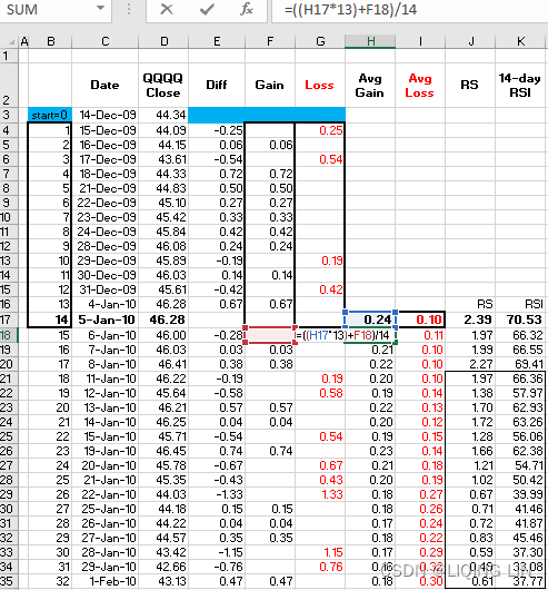
- Figure 9.12a shows that the profitability of the RSI reversed in about 1998. From 1970 to 1998 it was a good trend indicator; that is, when the RSI moved above 90 the S&P continued up. After 1998 it has been a much better mean-reverting indicator.
从 1970 年到 1998 年,它是一个很好的趋势指标; 也就是说,当 RSI 升至 90 上方时,标准普尔继续上涨。 1998 年之后,它成为一个更好的均值回归指标 - Figure 9.12b is the result of applying a method of scaling in to trades according to the following rules:

 FIGURE 9.12b A breakdown of longs and short sales using the scaling-in method, S&P 2000 through 2008.
On day t the RSI was 14 (<15), and we entered 50%, but then on day t + 1 the RSI dropped to 8; it was not clear whether we added an extra 25%, but we assume that is the case. Then the trade is exited if we do not add on the next day. Because the RSI can stay above or below 50 for long periods of time, an exit rule that waits for the RSI to cross 50 is not likely to be successful. Stokes’s approach of exiting after one day seems much safer. Figure 9.12b separates the longs and short sales from 2000 through 2008, showing that both sides performed well, a very desirable outcome. Having good performance for longs and shorts is not common because many markets have an upwards bias (especially the stock market). However, 1-day trades are sensitive to costs. Traders will need to see if the returns per share, or per contract, are suffi cient to cover commissions and slippage.
在 t 日,RSI 为 14,我们进入 50%,但随后在 t+1 日,RSI 降至 8; 目前尚不清楚我们是否额外增加了 25%,但我们假设是这样。 如果我们不在第二天添加,那么交易将退出。 由于 RSI 可以长时间保持在 50 以上或以下,因此等待 RSI 超过 50 的退出规则不太可能成功。 Stokes 在一天后退出的方法似乎更安全。 图 9.12b 将 2000 年至 2008 年的多头和空头销售分开,表明双方都表现良好,这是一个非常理想的结果。 多头和空头都有良好的表现并不常见,因为许多市场都有向上的偏见(尤其是股市)。 然而,1 日交易对成本很敏感。 交易者需要查看每股或每份合约的回报是否足以支付佣金和滑点。
A Standard 2-Period RSI
 FIGURE 9.13 2-Period RSI (center panel) compared with the traditional 14-day RSI (bottom panel), applied to NASDAQ futures, August 2005 through September 2008.
In Figure 9.13 a standard 2-period RSI is shown in the middle panel and the traditional 14-day RSI in the lower panel. Both are applied to NASDAQ futures, from August 2005 through September 2008, which appears at the top.
- The classic RSI penetrates the extremes of 30 and 70 but does not reach 20 or 80,
- while the 2-period RSI touches near 15 and 85 a number of times.
We might expect a 2-period oscillator to jump between 0 and 100 every day that prices changed direction, but the average-off calculation slows down the process and makes the 2-period chart a somewhat more volatile version of the standard RSI.
在图 9.13 中,标准的 2 周期 RSI 显示在中间面板中,传统的 14 天 RSI 显示在下面板中。 两者都适用于从 2005 年 8 月到 2008 年 9 月出现在顶部的纳斯达克期货。 经典 RSI 突破 30 和 70 的极端,但没有达到 20 或 80,而 2 周期 RSI 多次触及 15 和 85 附近。 我们可能期望 2 周期震荡指标每天在价格改变方向时在 0 和 100 之间跳跃,但average-off calculation减慢了该过程并使 2 周期图表成为标准 RSI 的更具波动性的版本。
An RSI Version of MACD
While the MACD creates a histogram of the difference between two moving averages, we can make that pattern easier to interpret by applying the RSI to the spread of the moving averages. In Figure 9.14 a 5-day RSI is applied to the difference between the 10- and 40-week moving average for the emini-S&P futures. Using the standard 30-70 thresholds, this seems to find credible points where prices are overbought and oversold.  FIGURE 9.14 RSI applied to the spread between a 10-week and 40-week moving average of
S&P futures.
Stochastics - momentum indicator
The stochastic indicator, created by George Lane, is an oscillator that measures the relative position of the closing price within a past high-low range. It is based on the commonly accepted observation that closing prices tend to resist penetrating the high prices of the past few days, the place where a horizontal resistance line would be drawn on a chart.它基于普遍接受的观察结果,即收盘价往往难以突破过去几天的高价,即图表上绘制水平阻力线的位置。 Similarly, in a downtrend prices must be able to close below the lows of the past few days for the move to continue. When the market is about to turn from up to down, for instance, it is often the case that the highs are higher than previous days, but the closing price settles nearer the low of the day, failing to indicate a continuation of the uptrend. This makes the stochastic oscillator different from the MACD, which uses the difference between two trends(2 EMA), and the RSI which uses only the closing prices. The stochastic uses the high, low, and close and unlike the other oscillators, there does not have to be any smoothing to introduce a lag.
The three indicators that result from the stochastic measurement are called %K, %D, and %D-slow. These indicators show increasingly slower interpretation of price movement, with %D being the most popular as a single indicator; however, %D and %D-slow are often used together to produce a trading signal. Calculation of these indicators for today’s value t over the past 5 days, are
- Fast Stochastic Oscillator(14,3),mpf11_4_plotly Align dual Yaxis_Chaikin/Stochastic Oscillator_ma Envelopes_support阻力_pivot point_KDJ_LIQING LIN的博客-CSDN博客
快速随机振荡器基于 George Lane 的 %K 和 %D 原始公式.%K 可能显得相当不稳定

for instances
Initial (raw)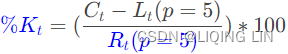

- Slow Stochastic Oscillator(14,3)慢速随机振荡器
2. While Fast Stochastic Oscillator is used for signals, the Slow Stochastic Oscillator is supposed to reflect this emphasis: 慢速随机震荡指标使用 3 天 SMA 平滑 %K,这正是快速随机震荡指标中的 %D
 #3 is a default smoothing period for getting slow K and slow D:
- Where
= today’s closing price
= the low price of the last 5 days
= the range of the last 5 days (highest high minus lowest low) as of today.
Calculating the Fast Stochastic Oscillator(14,3) for IBM
Fast Stochastic Oscillator(14,3),mpf11_4_plotly Align dual Yaxis_Chaikin/Stochastic Oscillator_ma Envelopes_support阻力_pivot point_KDJ_LIQING LIN的博客-CSDN博客
快速随机振荡器基于 George Lane 的 %K 和 %D 原始公式.%K 可能显得相当不稳定
![]()
for instances
Initial (raw) 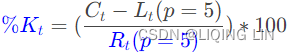

import numpy as np
import pandas as pd

def get_stochastic(df, window=14, fast_smoothing_p=3,
                   slow_smoothing_p=None,
                   stochastic='fast'
                  ):
    k_column = '%K_{}_fast'.format(window)
    d_column = '%D_{}_fast'.format(fast_smoothing_p)

    low_min= df['Low'].rolling(min_periods=1,
                               window=window,
                               center=False
                              ).min() # na in the first window-1 obs
    high_max = df['High'].rolling(min_periods=1,
                                  window=window,
                                  center=False
                                 ).max() # na in the first window-1 obs

    df[k_column] = (df['Close'] - low_min)/(high_max - low_min)*100
    df[d_column] =  df[k_column].rolling(min_periods=1,
                                         window=fast_smoothing_p,
                                         center=False,
                                        ).mean()

    if stochastic.lower() == 'slow' or stochastic.lower() == 'full' or slow_smoothing_p!=None:
        df.drop(columns=[k_column], inplace=True)
        new_k_column = ''
        if slow_smoothing_p!=None or stochastic.lower() == 'full':
            # Full Stochastic Oscillator(14,3,3)
            # 3. The Full Stochastic Oscillator is a fully customizable version of the Slow Stochastic Oscillator.
            # Users can set the look-back period of K,
            # the number of periods to slow %K,
            # and the number of periods for the %D moving average

            if slow_smoothing_p != None : # but stochastic.lower() == 'full'
                stochastic='full'
            elif stochastic.lower() == 'full': # but slow_smoothing_p!=None
                slow_smoothing_p = fast_smoothing_p
            # print(stochastic, slow_smoothing_p)
            new_k_column = '%K_{}_{}_{}'.format(window,
                                                slow_smoothing_p,
                                                stochastic.lower()
                                               )
        else: # Slow Stochastic Oscillator(14,3)
            slow_smoothing_p = fast_smoothing_p
            new_k_column = '%K_{}_{}'.format(window,
                                             stochastic.lower()
                                            )
        df.rename( columns={d_column:new_k_column},
                   inplace=True
                 )

        d_column_slow = '%D_{}_{}'.format(slow_smoothing_p, stochastic.lower())
        df[d_column_slow] =  df[new_k_column].rolling(min_periods=1,
                                                      window=slow_smoothing_p,
                                                      center=False,
                                                     ).mean()

    return df

import yfinance as yf

ibm = yf.download( 'ibm', start='2009-10-01', end='2010-05-01')
ibm = get_stochastic(ibm, window=14, fast_smoothing_p=3 )
ibm['2009-11-01':'2010-04-06'] 
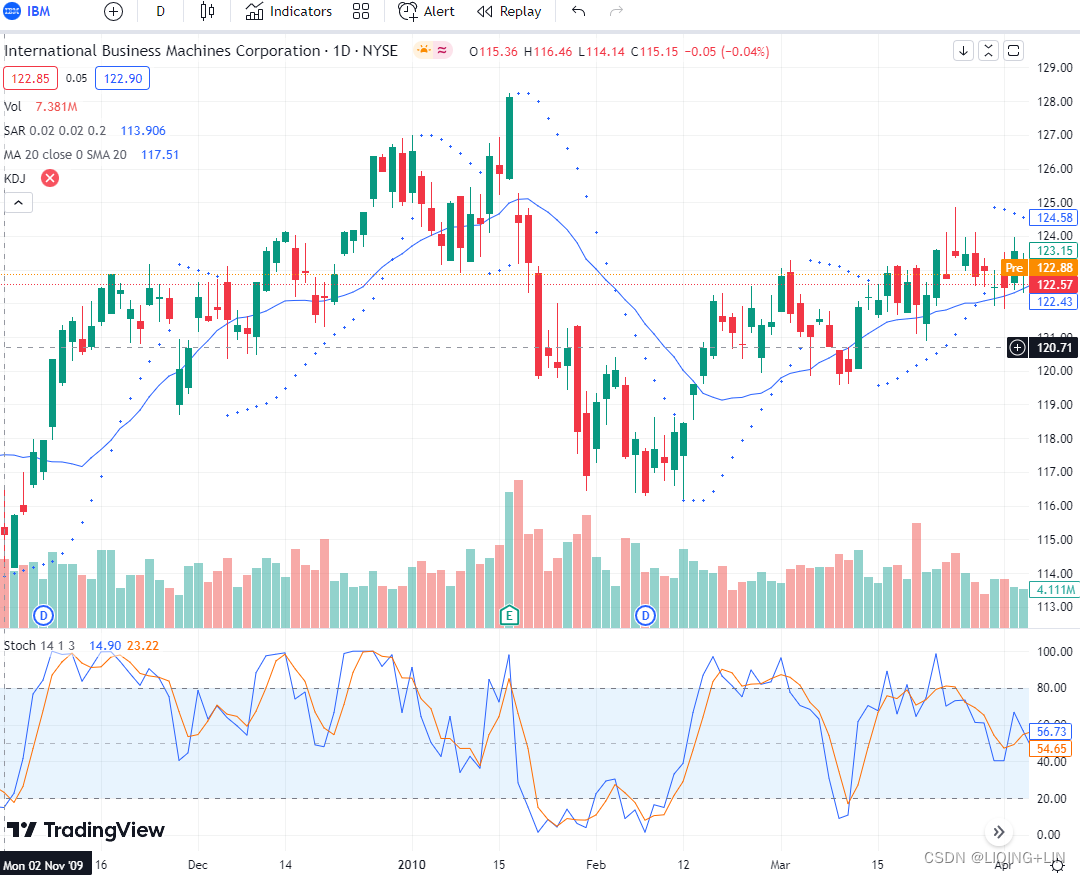

Calculating the Slow Stochastic Oscillator(14,3) for IBM
The default setting for the Stochastic Oscillator is 14 periods, which can be days, weeks, months or an intraday timeframe. A 14-period %K would use the most recent close, the highest high over the last 14 periods and the lowest low over the last 14 periods. %D is a 3-day simple moving average of %K. This line is plotted alongside %K to act as a signal or trigger line这条线与 %K 一起绘制,用作信号线或触发线.
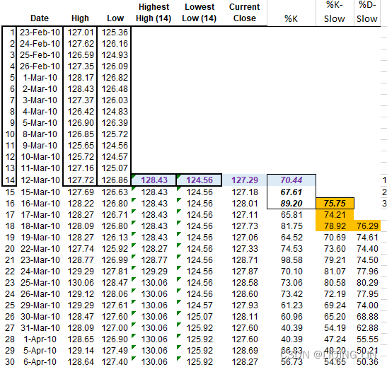
- 1. Highest High(14)
, the 14-day high using the function Max.
- 2. Lowest Low(14)
, the 14-day low using the function Min.
- 3. calculate the raw stochastic %K as

- 4.calculate the
 as
as 
- 5. calculate the
 as
as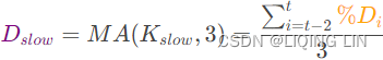
ibm = yf.download( 'ibm', start='2009-10-01', end='2010-05-01')
ibm = get_stochastic(ibm, window=14, fast_smoothing_p=3, stochastic='slow' )
ibm['2010-04-06':]
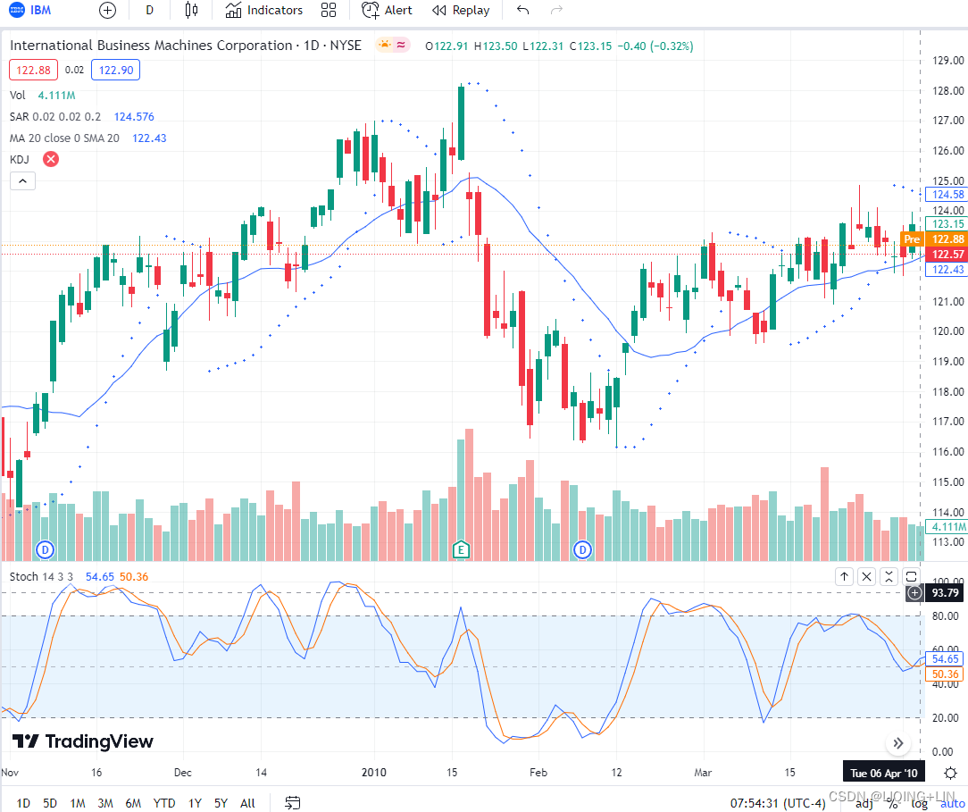
######
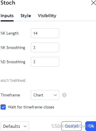 tradingview vs yahoo
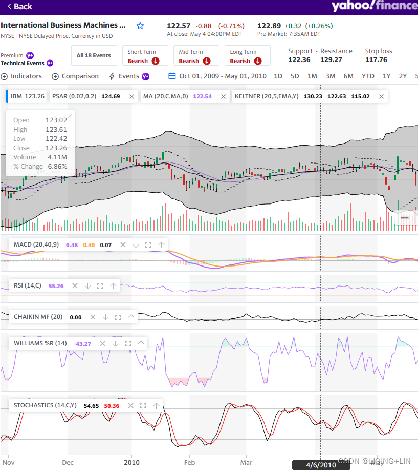
Calculating the Full Stochastic Oscillator(14,3, 3) for IBM
ibm = yf.download( 'ibm', start='2009-10-01', end='2010-05-01')
ibm = get_stochastic(ibm, window=14, fast_smoothing_p=3, slow_smoothing_p=3,
                     #stochastic='full'
                    )
ibm['2010-04-06':] 
Calculating the 10-Day Stochastic for Hewlett-Packard (HPQ)
The default setting for the Stochastic Oscillator is 10 periods, which can be days, weeks, months or an intraday timeframe. A 10-period %K would use the most recent close, the highest high over the last 14 periods and the lowest low over the last 14 periods. %D is a 3-day simple moving average of %K. This line is plotted alongside %K to act as a signal or trigger line这条线与 %K 一起绘制,用作信号线或触发线.
 The raw stochastic(%K) in column of the spreadsheet shows that values start above 90%(or 96.41) and drop to 6.07% in a few days. This happens when prices close near the highest or lowest prices of the past 10 days当价格收盘价接近过去 10 天的最高价或最低价时. When calculating the stochastic, today’s close is always included in the max, min, and range calculations. If today’s close price is the highest or lowest of the calculation period, then the raw stochastic will have a value of 100 or 0 如果今天的close价格是计算期间的最高价或最低价,则原始随机指标的值为 100 或 0
 .
. ![]()
![]() #3 is a default smoothing period for getting slow K and slow D:
#3 is a default smoothing period for getting slow K and slow D: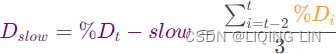
hpq = yf.download( 'hpq', start='2010-01-01', end='2011-01-29')
hpq = get_stochastic(hpq, window=10, fast_smoothing_p=3, #slow_smoothing_p=3,
                     stochastic='slow'
                    )
hpq['2011-01-01':] 
Comparing the Stochastic to Momentum and the RSI
The calculations for momentum, RSI, and the stochastic are very different; therefore, we would expect a chart of these indicators to vary considerably from one another. However, there are surprising similarities among the three, even calculated over the same 14-day period, 我们希望这些指标的图表彼此之间有很大差异。 然而,这三者之间有惊人的相似之处,即使是在相同的 14 天期间计算的 as shown in Figure 9.15.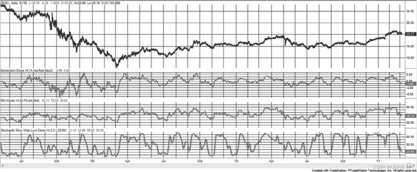 FIGURE 9.15 Comparison of simple momentum, RSI(middle), and stochastic(bottom), all for 14-day calculation periods, General Electric, May 2008 through February 2011.
The momentum and stochastic both show how today’s price relates to the prices over the calculation interval动量和随机指标都显示了今天的价格与计算区间内的价格之间的关系; therefore, we would expect them to be most similar, and that appears to be true. Both have peaks at the same place, although the %D-Slow stochastic has a smoother overall line due the two successive 3-day averages尽管 %D-Slow 随机指标由于两个连续的 3 天平均值而具有更平滑的整体线。.
The RSI chart does not seem to be lagged, instead it is dampened, appearing to have less volatility. In fact, the highs and lows rarely touch 70 and 30, while the stochastic highs and lows often go above 90 and below 10, even though it is smoothed. The overall impression of the stochastic is that it moves faster and exaggerates the swings随机指标的总体印象是它移动得更快并夸大了波动. 
Trading the Stochastic
Traditionally, the stochastic can be traded by using a combination of a slower and faster calculation to give signals, or by combining extreme stochastic values for entry or exit timing with a trend. To use the stochastic by itself, %D and %D-slow can take on the role of the faster indicator and the slower signal line in the same way as the MACD and its signal line were used. The fastest calculation, %K, is not often used due to its instability. Figure 9.16 shows the two 20-day calculations, %D and %D-slow, along the bottom of an S&P futures continuation chart from December 2001 through September 2002. A 60-day moving average is in the top panel. FIGURE 9.16 20-day stochastic (bottom) and a 60-day moving average for the S&P futures continuation series.
%D is a 3-day simple moving average of %K. This line is plotted alongside %K to act as a signal or trigger line这条线与 %K 一起绘制,用作信号线或触发线.
The downtrend in the S&P during 2002 produces two good sell signals using the stochastics. In March and August, the slower %D penetrates above the 80% threshold and crosses the signal line moving down. A third peak in May touches near 70% and would produce an additional sell signal if the upper threshold were set lower. During a sustained downtrend, it is common for the indicator values to fall below the lower threshold and remain there for extended periods. Although the rolling calculation is intended to self-adjust, the most practical solution is to combine the stochastic signals with a trend在持续下降趋势中,指标值通常会跌破下限并长时间保持在该水平。 虽然滚动计算的目的是自我调整,但最实用的解决方案是将随机信号与趋势结合起来.
The 60-day moving average, shown along with prices in the upper part of Figure 9.16, indicates a downtrend for the entire period of the chart. Using the relatively slow 20-day stochastic, the penetration of the upper 80% threshold gives very good timing for short sale entries, and avoids the problems of an unfavorable distribution of stochastic values. The 20-day stochastic does not indicate where to exit the downtrend. A faster stochastic can be used to produce more frequent sell signals that can be applied as follows
- Enter a short sale after the trend has turned down on the first stochastic sell signal(the stochastic crosses the signal line going down).
- Enter a long after the trend has turned up on the first stochastic buy signal.

The problem with all timing rules is that, if prices move higher and do not retrace, then there will not be a stochastic signal, or it will occur well after there would have been profits in the trade. Many of the lost opportunities can be eliminated by using a faster stochastic calculation period. It is particularly dangerous to use a timing rule for exiting a position. Delays in entering are lost opportunities, but delays exiting are real trading losses. 所有时间规则的问题在于,如果价格走高且不回撤,则不会出现随机信号,或者在交易获利后很久才会出现随机信号。 通过使用更快的随机计算周期可以消除许多失去的机会。 使用时间规则来退出仓位是特别危险的。 延迟进入是失去的机会,但延迟退出是真正的交易损失。
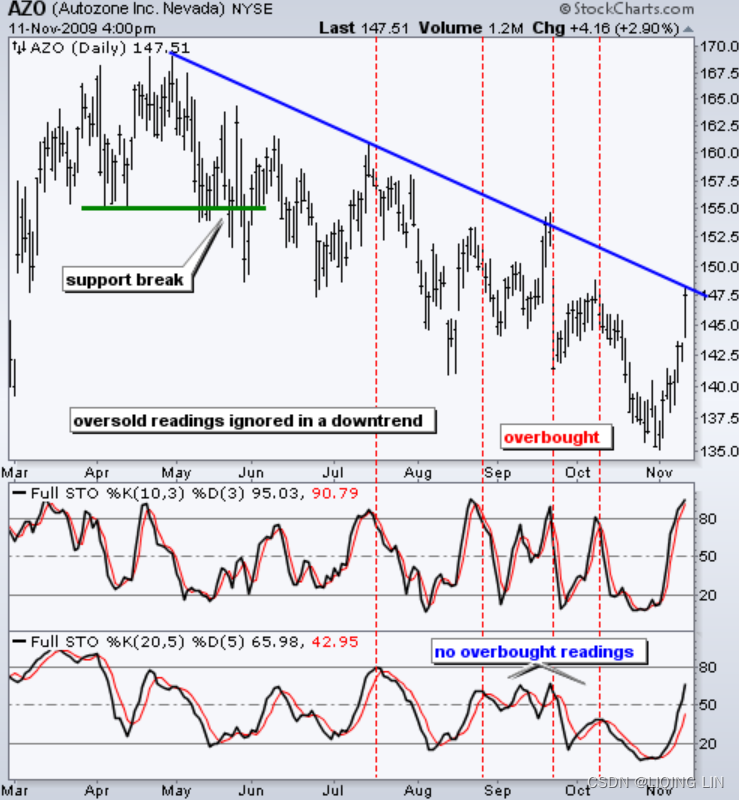
Chart 5 shows Autozone (AZO) with a support break in May 2009 that started a downtrend. With a downtrend in force, the Full Stochastic Oscillator (10,3,3) was used to identify overbought readings to foreshadow a potential reversal. Oversold readings were ignored because of the bigger downtrend. The shorter look-back period (10 versus 14) increases the sensitivity of the oscillator for more overbought readings. For reference, the Full Stochastic Oscillator (20,5,5) is also shown. Notice that this less sensitive version did not become overbought in August, September, and October. It is sometimes necessary to increase sensitivity to generate signals.
The settings on the Stochastic Oscillator depend on personal preferences, trading style and timeframe.
- A shorter look-back period(increases the sensitivity of the oscillator for more overbought readings) will produce a choppy oscillator震荡的振荡器 with many overbought and oversold readings.
- A longer look-back period(produce a less sensitive oscillator with fewer signals.) will provide a smoother oscillator with fewer overbought and oversold readings.
Left and Right Crossovers
The faster %K-slow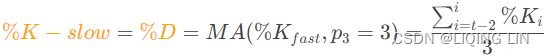 will usually change direction sooner than the %D-slow
 , crossing the %D-slow line while it is still moving in the prior trend direction. The opposite case, when the %D-slow turns first, indicates a slow, stable change of direction and is a more favorable pattern (Figure 9.17a). Using the fast %K-Slow and the slower %D-Slow, the following patterns have been identified:
- Hinge. A reduction in the speed of either the %K-slow or %D-slow lines, shown as a flattening out, indicates a reversal on the next day (Figure 9.17b).
%K-slow 或 %D-slow 线的速度降低,显示为变平,表明第二天出现反转 - Warning. An extreme turn in the faster %K-slow (from 2 to 12%) indicates at most two days remaining in the old trend.
faster %K-slow(从 2% 到 12%)的极端转变表明旧趋势最多还剩两天。 - Extremes. Reaching the extreme %K-slow values of 0 and 100 requires seven consecutive days of closes at the highs (or lows). The test of these extremes, following a pullback, is an excellent entry point.

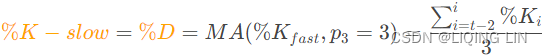
达到 0 和 100 的极端 %K-slow 值需要连续 7 天收于高点(或低点)。 在回调之后对这些极端的测试是一个很好的切入点。 - Set-up. Although the line chart(prices) shows higher highs and lows, if the %D-slow line has lower lows, a bear market set-up a has occurred. Look for a selling opportunity on the next rally (Figure 9.17c).
尽管折线图(prices)显示了更高的高点和低点,但如果 %D-慢线具有更低的低点,则熊市结构 a 已经发生。 在下一次反弹中寻找卖出机会
A bear set-up occurs when the price forms a higher low更高的波谷, but the Stochastic Oscillator forms a lower low更低的波谷.
(bearish divergence : The stock moved to higher highs更高的波峰, but the Stochastic Oscillator formed lower highs更低的波峰.)
Even though the stock held above its prior low, the lower low in the Stochastic Oscillator shows increasing downside momentum尽管该股保持在先前的低点之上,但随机震荡指标的较低低点显示下行势头在增加. The next advance is expected to result in an important peak预计下一个上涨将导致一个重要的可交易的高峰.
A bull set-up is basically the inverse of a bullish divergence
The underlying security price forms a lower high 更低的波峰, but the Stochastic Oscillator forms a higher high 更高的波峰.
(bullish divergence:stock moved to lower low 更低的波谷, but the Stochastic Oscillator formed a higher low 更高的波谷).
Even though the stock could not exceed its prior high, the higher high in the Stochastic Oscillator shows strengthening upside momentum. 尽管该股未能超过其先前的高点,但随机震荡指标较高的高点显示上行势头增强 The next decline is then expected to result in a tradable bottom预计下一次下跌将导致可交易的低谷.
- Failure. An excellent confi rmation of a change in direction occurs when %K-slow crosses %D-slow (after penetrating the extreme level), then pulls back to the %D-slow line, but fails to cross it again (Figure 9.17d).
当 %K-slow 穿过 %D-slow(在突破极限水平后),然后拉回到 %D-slow 线,但未能再次穿过它时,一个很好的方向变化确认发生
FIGURE 9.17 Lane’s patterns. (a) Left and right crossings. (b) Hinge. (c) Bear market set-up. (d) %K-slow failure.
(Stochastic RSI)Creating a Stochastic from the RSI
Any series or indicator value can be converted to a raw stochastic, %K , without adding lag by replacing the closing price with the indicator value. This creates a measure of where that indicator lies in its high-low range over the calculation period and may simplify the generation of buy and sell signals. A stochastic created from an RSI would bempf11_5_plotly_Keltner Channels_ATR_Stochastic RSI_%B MFI_LIQING LIN的博客-CSDN博客
The number of periods used to calculate StochRSI is transferred to RSI in the formula. For example, 14-day StochRSI would use the current value of 14-day RSI and the 14-day high-low range for 14-day RSI.
14-day StochRSI equals 0 when RSI is at its lowest point for 14 days.
14-day StochRSI equals 1 when RSI is at its highest point for 14 days.
14-day StochRSI equals .5 when RSI is in the middle of its 14-day high-low range.
14-day StochRSI equals .2 when RSI is near the low of its 14-day high-low range.
14-day StochRSI equals .80 when RSI is near the high of its 14-day high-low range.
import numpy as np
import pandas as pd

import numpy as np
import pandas as pd

def get_rsi(df, columnName='Adj Close',window=14):
    # https://pandas.pydata.org/docs/reference/api/pandas.Series.diff.html
    # Series.diff(default periods=1) # periods=1 : diff = current row - 1st previous row
    #                                # periods=3 : diff = current row - 3rd previous row
    #                                # periods=-1 : diff = current row - 1st following row
    df['Up Move'] = df[columnName].diff().apply(lambda diff: diff if diff>0 else 0)
    df['Down Move'] = df[columnName].diff().apply(lambda diff: -diff if diff<0 else 0)

    df['Average Up'] = np.nan
    df['Average Down'] = np.nan
    # Calculate initial Average Up & Down, RS and RSI
    # First Average Gain (Average price change on up days)
    df['Average Up'].iloc[window] = df['Up Move'].iloc[1:window+1].mean()     # 1 since df['Up Move'][0] is NaN  <== diff()

    # First Average Loss (Average price change on down days)
    df['Average Down'].iloc[window] = df['Down Move'].iloc[1:window+1].mean() # 1 since df['Down Move'][0] is NaN <== diff()


    # Relative Strength
    df['rs_{}'.format(window)] = np.nan
    # Relative Strength Index
    df['rsi_{}'.format(window)] = np.nan

    df['rs_{}'.format(window)].iloc[window] = df['Average Up'].iloc[window] / df['Average Down'].iloc[window]
    df['rsi_{}'.format(window)].iloc[window] = 100 - ( 100/(1+df['rs_{}'.format(window)].iloc[window]) )


    # Calculate rest of Average Up, Average Down, RS, RSI
    for row_index in range( window+1, len(df) ):

        df['Average Up'].iloc[row_index] = (df['Average Up'].iloc[row_index-1]*(window-1) +\
                                            df['Up Move'].iloc[row_index]
                                           )/window
        df['Average Down'].iloc[row_index] = (df['Average Down'].iloc[row_index-1]*(window-1) +\
                                              df['Down Move'].iloc[row_index]
                                             )/window
        df['rs_{}'.format(window)].iloc[row_index] = df['Average Up'].iloc[row_index] / df['Average Down'].iloc[row_index]
        df['rsi_{}'.format(window)].iloc[row_index] = 100 - (100/(1+df['rs_{}'.format(window)].iloc[row_index]))

    df.drop(columns=['Up Move','Down Move',
                     'Average Up','Average Down',
                     'rs_{}'.format(window)
                    ],
            inplace=True
           )
    return df


def get_stochrsi( df, window=14, cp='Close', n_sma=5 ):
    rsi_name='rsi_{}'.format(window)
    df = get_rsi(df, cp=cp, window=window)
    rsi = df[rsi_name]

    stochrsi_name = 'stochrsi_{}'.format(window)
    rsi_min = rsi.rolling(min_periods=1, window=window, center=False).min()
    rsi_max = rsi.rolling(min_periods=1, window=window, center=False).max()
    cv = (rsi - rsi_min) / (rsi_max - rsi_min)
    df[stochrsi_name]=cv*100

    sma_name='sma_{}_stochrsi_{}'.format(n_sma, window)
    df[sma_name] = df[stochrsi_name].rolling(min_periods=1, window=n_sma, center=False).mean()

    return df
Williams’s Oscillators
Larry Williams has been known for his development of trading methods based on oscillators since his publication of the A/D oscillatoin 1972. The three techniques described below have some similarities, even though the last one, the Ultimate Oscillator, was published 13 years later.
A/D Oscillator
In 1972, Jim Waters and Larry Williams published a description of their A/D Oscillator. For their method, A/D means accumulation/distribution rather than the popular notation of advance/decline, a well-known indicator for stocks. They used a unique form of relative strength, defining buying power(BP) and selling power(SP) as
- BP = High - Open
- SP = Close - Low
where the values used were today’s open, high, low, and closing prices. The two values, BP and SP, show the additional buying strength (relative to the open) and selling strength (compared to the close) in an effort to measure the implied direction of the day’s trading. This definition of buying and selling power is still used today.BP 和 SP 这两个值显示额外的买入强度(相对于开盘价)和卖出强度(相对于收盘价),以衡量当天交易的隐含方向。 The combined measurement, called the Daily Raw Figure (DRF) is calculated as
- The maximum value of 1 is reached when a market opens trading at the low and then closes at the high:
.
- When the opposite occurs and the market opens at the high and closes on the lows, the DRF = 0.
Each price series develops its own patterns, which can be smoothed or traded in many ways similar to a momentum index. The Waters-Williams A/D Oscillator solves problems of volatility and limit moves (although there are very few markets with trading limits any more) in futures markets (Waters-Williams A/D 振荡器解决了期货市场的波动和限价变动问题(尽管现在很少有交易限价的市场了)). DRF completely adjusts to higher or lower trading ranges because the divisor itself is a multiple of the day’s range. DRF完全调整到更高或更低的交易范围,因为除数本身是当天范围的倍数; because each day is treated independently, the cumulative values of the momentum index are not part of the results因为每一天都是独立处理的,所以动量指数的累积值不是结果的一部分.
This day-to-day evaluation has no memory and causes DRF to be very volatile, yet it still takes on the pattern of the underlying market. If fewer trades are preferred, the DRF can be smoothed.
The rules for using the A/D Oscillator were not defined in the original article, but some simple rules could be:
- • Sell when the DRF (or smoothed DRF) penetrates into the overbought zone. Close out all accumulated long positions (if any) and go short on the open of the next trading day.
当DRF(平滑的DRF) 进入超买区时卖出(卖出信号 直到DRF进入超卖区 才转为买入信号)。 平掉所有累积的多头头寸(如有)并在下一个交易日开盘时做空。 - • Buy and exit the short position when the opposite conditions occur.
- • All positions are entered on the next open after a signal. 所有仓位均在信号发出后的下一次开仓时入场。
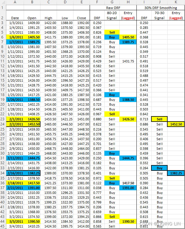 In the example in Table 9.2, a 0.30 exponential smoothing was used (selected arbitrarily) and the entry bands narrowed from 80-20 to 70-30 to reflect fewer extreme prices. Because the 1973 examples used soybeans, this example will do the same, but for 2011 data. Table 9.2 shows the calculations for the DRF and the smoothed DRF.
  FIGURE 9.18 A/D Oscillator.
The DRF is plotted as bars on a scale of 0 to 1.00 in Figure 9.18 and is extremely erratic非常不稳定. The solid line is the smoothed DRF. Once plotted, two horizontal lines can be drawn to isolate the peaks and bottoms of DRF; the top part becomes a zone representing an overbought condition, and the bottom zone represents oversold. For this chart, the 80-20 levels were used, although we expect this to be consistent over time because the range used in the denominator normalizes volatility. Even though we do not claim that these thresholds are predictive, the original article by Waters and Williams had lines drawn in a similar place. The thresholds for the smoothed DRF were set at 70-30.对于此图表,使用了 80-20 的水平,尽管我们预计这会随着时间的推移保持一致,因为分母中使用的范围使波动性正常化。 尽管我们并不声称这些阈值是可预测的,但 Waters 和 Williams 的原始文章在类似的地方画了线。 平滑 DRF 的阈值设置为 70-30。
For risk control, positions could be exited if the DRF does not post a lower value (for shorts) within one or two days, and the opposite for longs(为了风险控制,如果DRF在一两天内没有出现较低的价值(空头),则可以退出仓位,而多头则相反。). In Table 9.2 no stops were used. Long positions were held until a short signal occurred持有多头头寸直到出现空头信号, and shorts until a long was signaled并持有空头头寸直到发出多头信号. If the DRF (or smoothed DRF) enters an overbought or oversold zone more than once without the opposite zone being entered, an additional position can be added, although that was not done in the example.如果 DRF(或平滑 DRF)多次进入超买或超卖区域而没有进入相反区域,则可以添加额外的头寸,尽管在示例中没有这样做 Following these rules, the A/D Oscillator showed 9 trades, six of them profitable. For the smoothed DRF there were only 2 trades, both profitable. The amount of smoothing can easily be changed. For more signals, increase the smoothing constant so that it’s greater than 0.30对于更多信号,增加平滑常数,使其大于 0.30.
Although this example was very good, there are potential problems in the A/D Oscillator. The first happens on locked-limit days (where the market opens at the allowable limit and does not trade)限价锁定日(市场在允许的限价开盘并且不交易). In that case the open, high, low, and close are all the same and the DRF cannot be calculated because the divisor is zero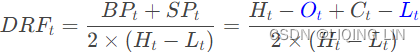 . Fortunately, there are few markets in which that can happen, but it did recently in cotton. A more basic problem concerns gap openings. A much higher opening with a stronger close would also upset the resulting DRF value.更高的开盘价和更强的收盘价也会扰乱最终的 DRF 值 Consider the following example:
 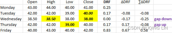 Note that on Wednesday, the DRF(the market opens at the high and closes on the lows, the DRF = 0) indicates that the momentum has reversed, but in fact the price is falling rapidly and gives no indication of recovering; it may actually be gaining momentum. On Thursday the price soars up and closes in the midrange, but the DRF shows a new downward momentum. The problem seems to be related to lack of association with the prior closing price. The daily movement can take on different appearances if the entire range was above or below the closing price(
Compare Closing price to yesterday's Closing price:
- If Close [today] > Close [yesterday]
Price Move [today] = Close [today] - True Range Low - If Close [today] < Close [yesterday]
Price Move [today] = Close [today] - True Range High - If Close [today] == Close [yesterday]
Price Move [today] = zero
).
- Example A: A small high/low range formed after a gap up
(the previous close is lower than the current low).
The TR equals the absolute value of the difference between the current high and the previous close. - Example B: A small high/low range formed after a gap down
(the previous close is greater than the current high).
The TR equals the absolute value of the difference between the current low and the previous close. - Example C: Even though the current close is within the previous high/low range, the current high/low range is quite small. In fact, it is smaller than the absolute value of the difference between the current high and the previous close, which is used to value the TR.
To form this link, replace the current high or low with the prior closing price, in the manner of the true range calculation, if that price was outside the current trading range如果该价格在当前交易范围之外,则以真实范围计算的方式用先前的收盘价替换当前的高点或低点. The following example shows that the results smoothed out and leaves the trend intact以下示例显示结果平滑并保持趋势不变。.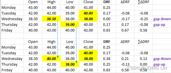
Linking the Current Day with the Prior Day
Another oscillator can be constructed using the highs and lows relative to the prior close:
The two days are linked together, and the ratio of the high price relative to the prior close is measured against the total range for the day. For the normal case, ; but if
replaces either
or
to extend the range, the value
will be either 1 or 0 for these extreme cases. As with the A/D Oscillator, the values derived from this method may also be smoothed.
Oscillators are not the only tools for measuring momentum or for determining overbought or oversold conditions. Because momentum is very different from either a charting technique or a moving average, it is valuable either on its own or as a confi rmation of another method.
A word of caution: Trading against the trend can be exciting and profitable逆势交易可能令人兴奋且有利可图, but at considerably greater risk than a trend-following system. The problem with selling an overbought condition is that it is much more difficult to hold losses to a minimum. A long position may be entered while prices are falling fast, and they may continue to fall at the same speed after you are long. Even a quick exit may sustain substantial losses.可能在价格快速下跌时进多头,你做多后可能继续以同样的速度下跌。 即使快速退出也可能蒙受重大损失。
Williams %R Method- momentum indicator
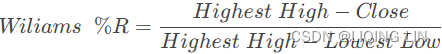 mpf11_3_status_plotly Align dual Yaxis_animation_button_MFI_Williams %Rsi_AO Co_VWAP_MAcd_BollingerB_LIQING LIN的博客-CSDN博客
After the publication of Williams’ How I Made One Million Dollars . . . Last Year . . . Trading Commodities, the %R oscillator became well known. It is a simple way of calculating where today’s closing price fi ts into the recent trading range. Using the last 10 days, define
Williams’ 10-day %R is different from 10-day stochastic , a because it measures how strong the market closed today compared to the high of the past 10 days. It is also conceptually upside down它在概念上也是颠倒的; that is, as the close gets stronger
 the value of %R gets smaller
. It may be intuitively easier to work with if you use 1.0 −%R. Williams viewed this as a timing device to add positions within a major technical or fundamental trend. This same approach was discussed with regard to the stochastic, and is shown in Figure 9.16. Trades were not entered if they contradicted the major market direction.如果交易与主要市场方向相矛盾,则不会进行交易
def get_wr(df, window=14):
    """ Williams Overbought/Oversold Index
    Definition: https://www.investopedia.com/terms/w/williamsr.asp
    WMS=[(Hn—Ct)/(Hn—Ln)] × -100
    Ct - the close price
    Hn - N periods high
    Ln - N periods low
    :param window: number of periods
    :return: None
    """
    column_name = 'wr_{}'.format(window)

    ln = df['Low'].rolling(min_periods=1,
                           window=window,
                           center=False
                          ).min()
    hn = df['High'].rolling(min_periods=1,
                            window=window,
                            center=False
                           ).max()

    df[column_name] = (hn - df['Close']) / (hn - ln) * -100
    return df
The Ultimate Oscillator(Momentum indicator)终极震荡指标
Ultimate Oscillator 由拉里·威廉姆斯 (Larry Williams) 于 1976 年开发,并于 1985 年刊登在《股票与商品》杂志上,是一种动量振荡器,旨在捕捉三个不同时间范围内的动量。 多时间框架目标旨在避免其他震荡指标的陷阱。 许多动量震荡指标在强势上涨开始时飙升,但随着上涨继续形成看跌背离。 这是因为他们受制于一个时间框架。 终极震荡指标试图通过在基本公式中加入更长的时间范围来纠正这个错误。 威廉姆斯确定了基于看涨背离的买入信号和基于看跌背离的卖出信号.
In the Ultimate Oscillator, Williams seems to combine his original idea of the A/D Oscillator with a great deal of Wilder’s RSI ( Larry Williams, “The Ultimate Oscillator,”Technical Analysis of Stocks & Commodities (August1985) ). He adds the unique feature of three concurrent time periods in order to offset the negative qualities of the short time period used for the %R, without slowing the system too much. The Ultimate Oscillator uses the following steps:
终极振荡器 (UO) 计算涉及很多步骤。 此示例基于默认设置 (7,14,28)。 首先,计算买入压力 (BP) 以确定价格走势的总体方向。 其次,测量相对于真实范围 (TR) 的购买压力。 这告诉我们收益或损失的真实大小。 第三,根据所涉及的三个时间范围 (7、14、28) 创建平均值。 第四,创建三个平均值的加权平均值。
- 1. Calculate today’s buying pressure
by subtracting the True Low from the Closing price,
. The True Low
.
which is the amount by which the close is above the "true low" on a given day. The true low is the lesser of the given day's trading low and the previous close.
买入压力 (BP) 衡量当前收盘价相对于当前低点或前收盘价的水平,以最低者为准 - 2. Calculate today’s true range,
The true range (the same as used in average true range) is the difference between the "true high" and the true low above. The true high is the greater of the given day's trading high and the previous close.
真实范围 (TR) 衡量从当前高点或前收盘价(以最高者为准)到 当前低点或前收盘价(以最低者为准)的价格范围. 买入压力和真实范围都包含了之前的收盘价,以说明从 一个时期 到 下一个时期 可能出现的差距Calculate the True Range (TR) which is the current period's high or the prior close, whichever is higher, minus the lowest value of the current period's low or the prior close. Record these values for each period as they will be summed up over the last 7, 14, and 28 periods to create TR Sum.
- 3. Total the Buying pressure
designated as,
, and
.
Total the true rangeover the same three periods,
通过将 BP 的 n个周期总和 除以 真实范围的 n个周期总和 来显示 相对于真实范围的买入压力。- The total buying pressure over the past 7 days is expressed as a fraction of the total true range over the same period. If
is today,
is yesterday, etc., then
- The total buying pressure over the past 7 days is expressed as a fraction of the total true range over the same period. If
- 4. Calculate the Ultimate Oscillator using the Average7, 14, and 28 values.
Average7 has a weight of 4, Average14 has a weight of 2, and Average28 has a weight of 1.(All three calculations are now in the same scale.)
Sum the weights in the denominator (in this case, the sum is seven, or 4+2+1). Multiply by 100 when other calculations are complete.
Notice that the nearest 7 values for the buying pressure and the true range are each used seven times(7=4+2+1), that is, they are multiplied by both the scaling factors of 4 and 2, and used once more in the 28-day calculation. Williams has created a step-weighted momentum, assigning values of 7, 3, and 1 to the first 7 days, second 7 days, and last 14 days, respectively. The last 14 days account for only 10% of the total. 
import numpy as np

def get_uo( df, fast_period = 7, medium_period=14, slow_period=28,
                fast_weight=4, medium_weight=2, slow_weight=1, ):
    # Validate arguments
    fast_period = int(fast_period) if fast_period and fast_period > 0 else 7
    fast_weight = float(fast_weight) if fast_weight and fast_weight > 0 else 4.0

    medium_period = int(medium_period) if medium_period and medium_period > 0 else 14
    medium_weight = float(medium_weight) if medium_weight and medium_weight > 0 else 2.0

    slow_period = int(slow_period) if slow_period and slow_period > 0 else 28
    slow_weight = float(slow_weight) if slow_weight and slow_weight > 0 else 1.0

    df['TrueLow'] = pd.DataFrame(dict(enumerate([ df['Low'],
                                                  df['Close'].shift(1),
                                                ])
                                    )
                               ).apply( min,axis=1 )
    df['TrueHigh'] = pd.DataFrame(dict(enumerate([ df['High'],
                                                   df['Close'].shift(1),
                                                 ])
                                    )
                               ).apply( max,axis=1 )
    df.loc[df.index[0],[ 'TrueLow', 'TrueHigh'] ]=np.nan # since df['Close'].shift(1)

    # buying pressure
    df['BP'] = df['Close'] - df['TrueLow']
    # true range
    df['TR'] = df['TrueHigh'] - df['TrueLow']

    df['fast_avg'] = df['BP'].rolling(window=fast_period).sum() / df['TR'].rolling(window=fast_period).sum()
    df['medium_avg'] = df['BP'].rolling(window=medium_period).sum() / df['TR'].rolling(window=medium_period).sum()
    df['slow_avg'] = df['BP'].rolling(window=slow_period).sum() / df['TR'].rolling(window=slow_period).sum()

    # Ultimate Oscillator
    total_weight = fast_weight + medium_weight + slow_weight
    SB = df['fast_avg']*fast_weight + df['medium_avg']*medium_weight + df['slow_avg']*slow_weight
    df['UO_{}_{}_{}'.format(fast_period,
                            medium_period,
                            slow_period
                           )
      ] = 100 * SB / total_weight
    df.drop(columns=['TrueLow', 'TrueHigh',
                     'BP','TR','fast_avg', 'medium_avg', 'slow_avg'# comment out this line
                    ],
            inplace=True)
    return df

mon = pd.read_excel('cs-ultosc.xlsx',
                    sheet_name='ultimate oscillator',
                    header=4,
                    index_col=2
                   )

mon = get_uo( mon.loc[ :,['High','Low','Close'] ],
              fast_period = 7, medium_period=14, slow_period=28,
              fast_weight=4, medium_weight=2, slow_weight=1
            )
mon
aapl = yf.download( 'aapl', start='2013-01-01', end='2018-12-31')
aapl = get_uo( aapl.loc[ :,['High','Low','Close'] ],
               fast_period = 7, medium_period=14, slow_period=28,
               fast_weight=4, medium_weight=2, slow_weight=1
             )
aapl.iloc[:30] 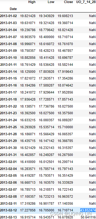
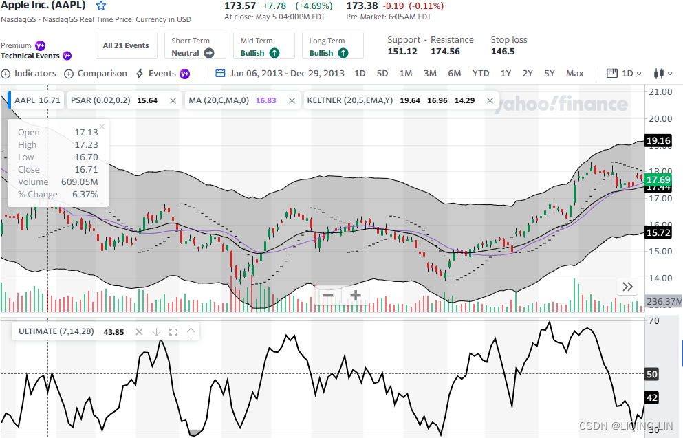
The rules for using this oscillator (Figure 9.19) are:
- 1. A sell set-up occurs when the oscillator moves above the 50% line, peaks at a high value, declines, and then moves higher. If the oscillator fails to move above the peak on the next rally/ ˈræli /(尤指股价)止跌回升, a short sale order can be placed when the oscillator fails on the right shoulder. This is a traditional top confirmation signal.
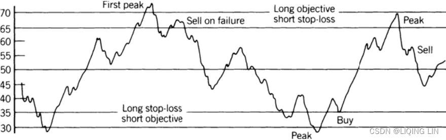 FIGURE 9.19 Williams’ Ultimate Oscillator.
 - 2. Short positions are closed out when a long signal occurs, when the 30% level is reached, or if the oscillator rises above 65% (the stop-loss point) after being below 50%.
- 3. A buy signal is given using the opposite formation as the short signal (rule 1).使用与空头信号相反的形态给出买入信号(规则 1)
- 4. Close out longs when a short signal occurs, when the 70% level is reached, or if the oscillator falls below 30% (after being above 50%).
KEY TAKEAWAYS
- The indicator uses three timeframes in its calculation: 7, 14, and 28 periods.
- The shorter timeframe has the most weight in the calculation, while the longer timeframe has the least weight.
- Buy signals occur when there is bullish divergence, the divergence low is below 30 on the indicator, and the oscillator then rises above the divergence high.
- A sell signal occurs when there is bearish divergence, the divergence high is above 70, and the oscillator then falls below the divergence low.
Interpretation
Buying Pressure and its relationship to the True Range
forms the base for the Ultimate Oscillator. Williams believes that the best way to measure Buying Pressure is simply subtracting the Close from the Low or the Prior Close, whichever of the two is the lowest. This will reflect the true magnitude of the advance, and hence, buying pressure.这将反映前进的真实幅度,从而反映购买压力。 The Ultimate Oscillator rises when Buying Pressure is strong and falls when Buying Pressure is weak. 终极震荡指标在买入压力强时上升,在买入压力弱时下降
The Ultimate Oscillator measures momentum for three distinct timeframes. Notice that the second timeframe is double that of the first, and the third timeframe is double that of the second. Even though the shortest timeframe carries the most weight(4), the longest timeframe is not ignored, which should reduce the number of false divergences这应该会减少虚假背离的数量. This is important because the basic buy signal is based on a bullish divergence and the basic sell signal is based on a bearish divergence.
Buy Signal
There are three steps to a buy signal.
- First, a bullish divergence forms between the indicator and security price. This means the Ultimate Oscillator forms a higher low as price forges a lower low. The higher low in the oscillator shows less downside momentum振荡器中较高的低点表明下行势头较小.
- Second, the low of the bullish divergence should be below 30. This is to ensure that prices are somewhat oversold or at a relative extremity.
看涨背离的低点应低于 30(这里说的是指标必须先<30阀值 然后再 >30形成higher low)。这是为了确保价格略微超卖或处于相对极端。 - Third, the oscillator rises above the high of the bullish divergence.
第三,升至看涨背离的高点之上(>70阀值)。背离高点是背离的两个低点之间的高点。
Chartists could have used the move above 50(>50) as a trigger for the Ultimate Oscillator instead.
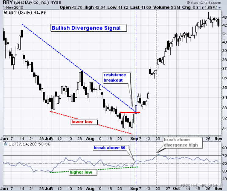 Best Buy (BBY) is shown with the Ultimate Oscillator (7,14,28) becoming oversold(<30) in late June and forming a large bullish divergencewith a higher low in late August. Technically, the indicator did not confirm the divergence until mid-September. Technical analysis, however, requires a little flexibility. Chartists could have used the move above 50(>50) as a trigger for the Ultimate Oscillator instead. This centerline acts as a bull-bear threshold for the indicator. The cup is half full (bullish bias) when above and half empty (bearish bias) when below在杯子半满的上方时是看涨偏见(超过半个杯子),在半空的下方时是看跌偏见(低于半个杯子) Also notice that the stock broke the June trend line and surged above short-term resistance in early September for further confirmation.
 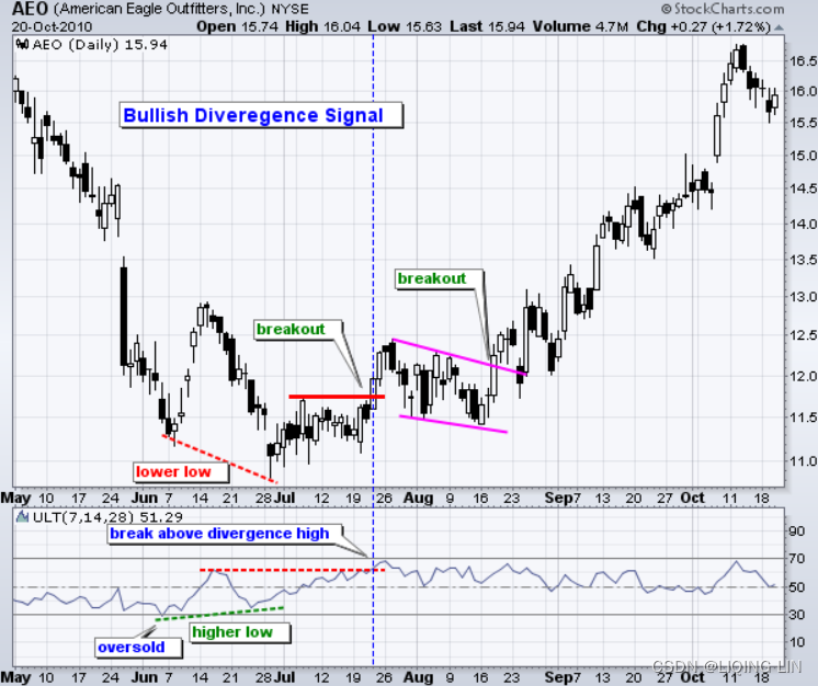 The chart shows American Eagle (AEO) with a smaller bullish divergence signal. The Ultimate Oscillator moved to oversold levels (<30) as the stock fell in early June. While the stock moved to new lows in late June, the indicator held above its prior low and above 30(>30). The subsequent break above the intermittent/ ˌɪntərˈmɪtənt /间歇的,断断续续的 high confirmed the bullish divergence signal(> 70). Also notice that AEO broke above resistance with a four-day surge. Even those who missed the breakout got a second chance as the stock pulled back in August and again broke resistance.另请注意,AEO 连续四天飙升突破阻力位。 甚至那些错过突破的人也获得了第二次机会,因为该股在 8 月回落并再次突破阻力位。
Sell Signal
There are three steps to a sell signal.
- First, a bearish divergence forms between the indicator and security price. This means the Ultimate Oscillator forms a lower high as price forges a higher high. The lower high in the oscillator shows less upside momentum.
这是当价格创下更高的高点但指标处于更低的高点时。 - Second, the high of the bearish divergence should be above 70. This is to ensure that prices are somewhat overbought or at a relative extremity.
看跌背离的高点应低于 70(这里说的是指标必须先>70阀值 然后再 <70形成higher low)。这是为了确保价格略微超买或处于相对极端。 - Third, the oscillator falls below the low of the bearish divergence to confirm a reversal.
第三,终极震荡指标必须跌破背离低点。 背离低点是背离的两个高点之间的低点。
 Caterpillar surged to a new high in late April, but the Ultimate Oscillator failed to confirm this high and formed a lower high. Also, notice that the indicator became overbought(>70) in mid-April. The subsequent break below the divergence low(< 50) in late April confirmed the bearish signal. CAT broke trend line support two days later and declined sharply into early June.
 The chart above shows Starbucks with an unconfirmed bearish signal and then a confirmed signal. The Ultimate Oscillator became overbought(>70) in the latter part of April. As the stock moved to new highs, the indicator forged lower highs in mid-May and again in late June. A bearish divergence was working in mid-May, but the indicator never broke its divergence low for confirmation(never < 50). After a bigger divergence formed, the indicator broke its divergence low(< 50) at the end of June to foreshadow a rather sharp decline.
The Difference Between the Ultimate Oscillator and Stochastic Oscillator
The Ultimate Oscillator has 3 lookback periods or timeframes. The Stochastic Oscillator has only 1.
![]()

![]()
![]()
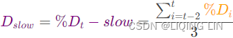
The Ultimate Oscillator doesn't typically include a signal line (one could be added), while the Stochastic does. While both indicators generate trade signals based on divergence, the signals will be different due to the different calculations. Also, the Ultimate Oscillator uses a three-step method for trading divergence.
Limitations of Using the Ultimate Oscillator
While the three-step trading method for the indicator may help eliminate some poor trades, it also eliminates many good ones. Divergence is not present at all price reversal points. Also, a reversal won't always occur from overbought or oversold territory. Also, waiting for the oscillator to move above the divergence high (bullish divergence) or below the divergence low (bearish divergence) could mean poor entry point as the price may have already run significantly in the reversal direction等待振荡器移动至背离高点(看涨背离)上方或背离低点(看跌背离)下方可能意味着切入点不佳,因为价格可能已经在反转方向上大幅运行。.
As with all indicators, the Ultimate Oscillator shouldn't be used in isolation, but rather as part of a complete trading plan. Such a plan will typically include other forms of analysis such as price analysis, other technical indicators, and/or fundamental analysis.
Timeframes
The Ultimate Oscillator can be used on intraday, daily, weekly or monthly charts. It is sometimes necessary to adjust the parameters to generate overbought or oversold readings, which are part of the buy and sell signals. Relatively docile stocks or securities may not generate overbought or oversold readings相对温顺的股票或证券可能不会产生超买或超卖读数 with the default parameters (7,14,28). Chartists need to increase sensitivity with shorter timeframes. The chart for Boeing (BA) shows the Ultimate Oscillator (7,14,28) trading between 30 and 70 for six months. There were no overbought or oversold readings没有超买或超卖读数. Shortening the timeframe to (4,8,16) increased sensitivity and generated at least six overbought or oversold readings将时间范围缩短至 (4,8,16) 会增加灵敏度并生成至少六个超买或超卖读数. The opposite is true for securities with high volatility高波动性证券的情况正好相反. It is sometimes necessary to lengthen the timeframes to reduce sensitivity and the number of signals有时需要延长时间范围以降低灵敏度和信号数量.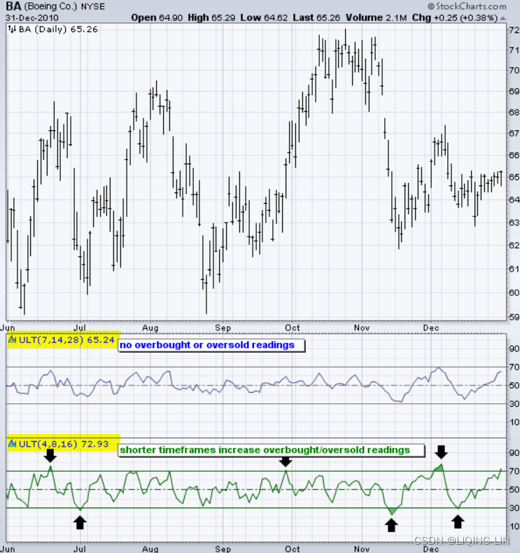
Conclusion
The Ultimate Oscillator is a momentum oscillator that incorporates three different timeframes. Traditional signals are derived from bullish and bearish divergence, but chartists can also look at actual levels for a trading bias. This usually works better with longer parameters and longer trends. For example, the Ultimate Oscillator (20,40,80) and price trend favors the bulls when above 50 and the bears when below 50但图表师也可以查看实际水平以寻找交易偏差。 这通常适用于更长的参数和更长的趋势。 例如,终极震荡指标 (20,40,80) 和价格趋势在高于 50 时有利于多头,在低于 50 时有利于空头。. As with all indicators, the Ultimate Oscillator should not be used alone. Complementary indicators, chart patterns and other analysis tools should be employed to confirm signals.
(RVI, RVgI momentum indicator)Relative Vigor Index 相对活力指数
John Ehlers, who has contributed extensively in the mathematical analysis of prices, in particular using cycles, has created the Relative Vigor Inde(RVI), a very smoothed momentum indicator(that measures the strength of a trend by comparing a security's closing price to its trading range while smoothing the results using a simple moving average (SMA).).(John F. Ehlers, “Relative Vigor Index,” Technical Analysis of Stocks & Commodities (January 2002).) The basic form of RVI is
However, the final RVI uses a 4-day symmetric weighting (similar to a triangular weighting) of the close − open in the numerator, and a similar symmetric weighting of the high − low in the denominator.
RVI is conceptually similar to the A/D Oscillator; however, the RVI is smoothed in a special way that targets a particular price cycle and eliminates the 2-bar cycle and its associated unwanted frequencies. RVI 以一种特殊的方式进行了平滑处理,该方式针对特定的价格周期并消除了 2 条柱线周期 及其相关的不需要的频率。 While it is preferable that the price series be analyzed for its cycle period, Ehlers suggests using 10 as the nominal value.虽然最好按周期分析价格序列,但 Ehlers 建议使用 10 作为名义值。 The RVI is calculated as
Numerator at time t
Denominator at time t
while
OR while
RVI signal line at time t
where ,
,
, and
are today’s Open, High, Low, and Closing prices and m is the calculation period, nominally 10.
import numpy as np
from math import floor

def symmetric_triangle(n, **kwargs):
    """Symmetric Triangle with n >= 2
    Returns a numpy array of the nth row of Symmetric Triangle.
    n=4  => triangle: [1, 2, 2, 1]
         => weighted: [0.16666667 0.33333333 0.33333333 0.16666667]
    """
    # https://numpy.org/doc/stable/reference/generated/numpy.fabs.html
    # fabs(x): Compute the absolute values element-wise.
    # This function returns the absolute values (positive magnitude) of the data in x.
    # Complex values are not handled, use absolute to find the absolute values of complex data.
    n = int( np.fabs(n) ) if n is not None else 2

    triangle = None
    if n == 2:
        triangle = [1, 1]

    if n > 2:
        if n % 2 == 0:
            front = [ i + 1
                      for i in range( 0, n //2 )
                    ] # if n==4 and n//2=2, then front =[1,2]
            triangle = front + front[::-1] # [1,2] + [2,1] ==> [1,2,2,1]
        else:
            front = [ i + 1
                      for i in range( 0, (n+1)//2 ) #(n+1)//2 hidden: round up
                    ]# if n==5 and 0.5*(5+1)=3 , then front=[1,2,3]
            triangle = front.copy()
            front.pop(-1)
            triangle += front[::-1] # [1,2,3] + [2,1] ==> [1,2,3,2,1]

    # if kwargs.pop("weighted")== True and triangle is a list:
    # Note: defatul False in the kwargs.pop("weighted", False), if weighted not exist return the default value
    if kwargs.pop("weighted", False) and isinstance(triangle, list):
        triangle_weights = triangle / np.sum(triangle) # [1,2,2,1]/6.
        return triangle_weights # array([1/6.,2/6.,2/6.,1/6.]) or array([0.16666667, 0.33333333, 0.33333333, 0.16666667])

    return triangle # [1,2,2,1] or [1,2,3,2,1]

def swma(close, lookback_period=None, offset=None, **kwargs):
    """Indicator: Symmetric Weighted Moving Average (SWMA)"""
    # Validate Arguments
    length = int(lookback_period) if lookback_period and lookback_period > 0 else 10

    if close is None: return

    # Calculate Result
    triangle = symmetric_triangle( lookback_period, weighted=True )
    # if lookback_period==4 and weighted=True
    #  then triangle==[1/6,2/6,2/6,1/6]

    # https://pandas.pydata.org/docs/reference/api/pandas.core.window.rolling.Rolling.apply.html
    # raw=True : the passed function will receive ndarray objects instead.
    #            If you are just applying a NumPy reduction function this will achieve much better performance.
    # raw=False: passes each row or column as a Series to the function.
    swma = close.rolling( lookback_period,
                          min_periods=lookback_period
                        ).apply( lambda rolling_window : np.dot(rolling_window,
                                                                triangle
                                                               )
                               )
    #    then swma = np.dot( [ close[t], close[t-1], close[t-2], close[t-3] ],
    #                        [1/6,2/6,2/6,1/6]
    #                      )

    return swma

def get_rvi(df, swma_lookback_period=4, window=10,):
    """Indicator: Relative Vigor Index (RVGI)"""
    window = int(window) if window and window > 0 else 10

    # swma : Symmetric Weighted Moving Average
    swma_lookback_period = int(swma_lookback_period) if swma_lookback_period and swma_lookback_period > 0 else 4

    numerator = swma( df['Close']-df['Open'],
                      lookback_period=swma_lookback_period,
                      weighted=True
                    ).rolling(window).sum()
    denominator = swma( df['High']-df['Low'],
                      lookback_period=swma_lookback_period,
                      weighted=True
                    ).rolling(window).sum()

    df['rvi_{}_{}'.format(swma_lookback_period, window)] = numerator/denominator
    df['rvi_signal_{}'.format(swma_lookback_period)] = swma( df[ 'rvi_{}_{}'.format(swma_lookback_period,
                                                                                    window
                                                                                   )
                                                               ],
                                                             lookback_period=swma_lookback_period,
                                                             weighted=True
                                                           )
    df['rvi_hist']=df['rvi_{}_{}'.format(swma_lookback_period, window)]-df['rvi_signal_{}'.format(swma_lookback_period)]
    return df

aapl = yf.download( 'aapl', start='2013-01-01', end='2018-12-31')
rvi_n=10
swma_n=4
aapl= get_rvi( aapl, swma_lookback_period=swma_n, window=rvi_n,)
aapl.iloc[:swma_n+rvi_n+swma_n]
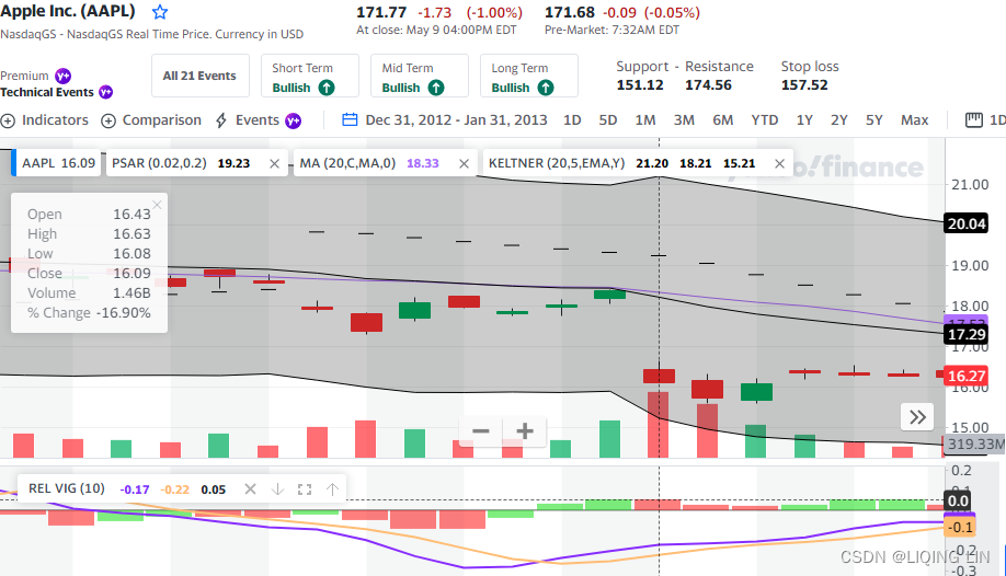
The RVI signal line is used in the same manner as the MACD signal line. After a peak in the RVI value, showing an overbought situation, the sell signal occurs the first time that the RVI crosses the RVI signal line moving lower.
The RVI's usefulness is based on the observed tendency for prices to close higher than they open during uptrends, and to close lower than they open in downtrends.
- The Relative Vigor Index (RVI) is a technical momentum indicator.
- The RVI oscillates across a pre-determined center line rather than a banded trend.
RVI 在预先确定的中心线而不是带状趋势上振荡 - Divergences between the RVI indicator and price suggest there will be a near-term change in the trend.
RVI 指标和价格之间的背离表明趋势将在近期发生变化。
What Does the Relative Vigor Index (RVI) Tell You?
The RVI indicator
Numerator at time t
Denominator at time t
is calculated in a similar fashion to the stochastics oscillator(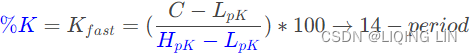 ) but it compares the close relative to the open rather than comparing the close relative to the low. Traders expect the RVI value to rise as the bullish trend gains momentum because, in this positive setting, a security's closing price tends to be at the top of the range while the open is near the low of the range.
The RVI is interpreted in the same way as many other oscillators, such as moving average convergence-divergence (MACD) or the relative strength index (RSI). While oscillators tend to fluctuate between set levels, they may remain at extreme levels over a prolonged period of time so that interpretation must be undertaken in a broad context to be actionable.虽然震荡指标往往在设定水平之间波动,但它们可能会在很长一段时间内保持在极端水平,因此必须在广泛的背景下进行解释才能采取行动。
The RVI is instead a centered oscillator and not a banded (trend-following) oscillator, which means that it's typically displayed above or below the price chart, moving around a center line rather than the actual price. It's a good idea to use the RVI indicator in conjunction with other forms of technical analysis in order to find the highest probability outcomes.
Example of How To Use the Relative Vigor Index (RVI)
A trader might examine potential changes in a trend with the RVI indicator by looking for divergences with the current price and then identifying specific entry and exit points with traditional trendlines and chart patterns.
交易者可以通过寻找与当前价格的背离,然后使用传统趋势线和图表模式识别特定的进入点和退出点,从而使用 RVI 指标检查趋势的潜在变化。
The two most popular trading signals include:
- RVI Divergences: Divergence between the RVI indicator and price suggests there will be a near-term change in the trend in the direction of the RVI's trend. So, if a stock price is rising and the RVI indicator is falling, it predicts the stock will reverse over the near term.如果股价上涨而 RVI 指标下跌,则预测该股将在短期内反转。
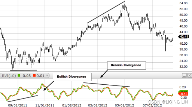
- RVI Crossovers: Like many oscillators, the RVI has a signal line that's often calculated with price inputs. A crossover above the signal line is a bullish indicator, while a crossover below the signal line is a bearish indicator. These crossovers are designed to be leading indicators of future price direction.交叉信号线向上是看涨指标,而交叉信号线向下是看跌指标。 这些交叉旨在成为未来价格方向的领先指标。
 In up trends potential buy opportunities occur when the RVI crosses above its signal line.
Limitations of Using the Relative Vigor Index (RVI) 使用相对活力指数 (RVI) 的局限性
The RVI works best in trending markets and tends to generate false signals in rangebound markets. Results can be improved by setting longer-term lookback periods, which help to reduce the impact of whipsaws and short-term countertrends.RVI 在趋势市场中效果最好,在区间波动市场中往往会产生错误信号。 可以通过设置更长期的回顾期来改善结果,这有助于减少洗盘和短期逆势的影响。


 1万+
1万+


 被折叠的 条评论
为什么被折叠?
被折叠的 条评论
为什么被折叠?
 到【灌水乐园】发言


