《Multi-Level Wavelet Convolutional Neural Networks》阅读笔记

最新推荐文章于 2025-03-06 10:09:12 发布

6个小石头

最新推荐文章于 2025-03-06 10:09:12 发布

阅读量6.5k

点赞数 6

分类专栏：阅读论文文章标签：图像去噪 MWCNN

本文链接：https://blog.csdn.net/LiuJiuXiaoShiTou/article/details/106135647

版权

本文介绍了多级小波卷积神经网络（MWCNN）在图像去噪、超分辨率和JPEG伪影去除等任务中的应用。MWCNN通过将小波变换嵌入CNN架构，避免了信息丢失，提高了接收场大小和计算效率的平衡。实验表明，MWCNN在多种图像恢复任务上表现出优越性能，同时避免了传统方法如扩张滤波的网格化副作用。

摘要生成于 C知道，由 DeepSeek-R1 满血版支持，前往体验 >

一、论文

《Multi-Level Wavelet Convolutional Neural Networks》

摘要：在计算机视觉中，卷积网络（CNN）通常采用合并来扩大接收域，其优点是计算复杂度低。但是，合并可能导致信息丢失，因此不利于进一步的操作，例如特征提取和分析。最近，已经提出了扩张滤波器来在接收场大小和效率之间进行折衷。但是，伴随的网格化效果可能导致对具有棋盘格图案的输入图像进行稀疏采样。为了解决这个问题，在本文中，我们提出了一种新颖的多级小波CNN（MWCNN）模型，以在接收场大小和计算效率之间取得更好的折衷。核心思想是将小波变换嵌入CNN架构中，以降低特征图的分辨率，同时增加接收场。具体来说，用于图像恢复的MWCNN基于U-Net架构，并且部署了逆小波变换（IWT）来重建高分辨率（HR）特征图。提出的MWCNN也可以看作是对扩张滤波器的改进和对平均池化的概括，并且不仅可以应用于图像恢复任务，而且可以应用于需要池化操作的任何CNN。
实验结果证明了所提出的MWCNN在诸如图像去噪，单图像超分辨率，JPEG图像伪影去除和对象分类等任务上的有效性。

二、网络结构

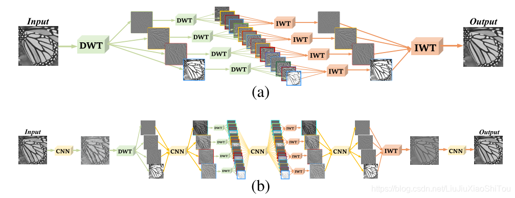
从WPT到MWCNN。直观地讲，WPT可以看作是我们的MWCNN的特例，没有（a）和（b）所示的CNN块。通过将CNN块插入WPT，我们将MWCNN设计为（b）。显然，我们的MWCNN是多级WPT的概括，当每个CNN块成为身份映射时，将其简化为WPT。

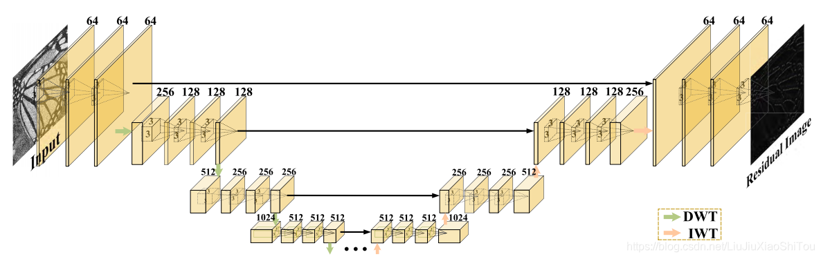
图3.多级小波CNN架构。它由两部分组成：收缩和扩展子网。每个实体框对应一个多通道要素图。通道数标注在框的顶部。卷积层数设置为24。此外，通过复制第三级子网的配置，我们的MWCNN可以进一步扩展到更高的级别。

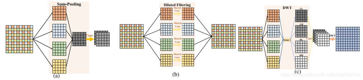
图4.平均池，膨胀滤波器和建议的MWCNN的图示。以一个CNN块为例：（a）因数为2的求和合并会导致最显着的信息丢失，不适合图像恢复；（b）速率为2的膨胀滤波等于子图像上的共享参数卷积；（c）拟议的MWCNN首先将图像分解为4个子带，然后将它们合并为CNN块的输入。然后，将IWT用作上采样层以恢复图像的分辨率。

三、代码

代码下载：https://github.com/lpj-github-io/MWCNNv2/tree/master/MWCNN_code

from model import common
import torch
import torch.nn as nn
import scipy.io as sio

def make_model(args, parent=False):
    return MWCNN(args)

class MWCNN(nn.Module):
    def __init__(self, args, conv=common.default_conv):
        super(MWCNN, self).__init__()
        n_resblocks = args.n_resblocks
        n_feats = args.n_feats
        kernel_size = 3
        self.scale_idx = 0
        nColor = args.n_colors

        act = nn.ReLU(True)

        self.DWT = common.DWT()
        self.IWT = common.IWT()

        n = 1
        m_head = [common.BBlock(conv, nColor, n_feats, kernel_size, act=act)]
        d_l0 = []
        d_l0.append(common.DBlock_com1(conv, n_feats, n_feats, kernel_size, act=act, bn=False))


        d_l1 = [common.BBlock(conv, n_feats * 4, n_feats * 2, kernel_size, act=act, bn=False)]
        d_l1.append(common.DBlock_com1(conv, n_feats * 2, n_feats * 2, kernel_size, act=act, bn=False))

        d_l2 = []
        d_l2.append(common.BBlock(conv, n_feats * 8, n_feats * 4, kernel_size, act=act, bn=False))
        d_l2.append(common.DBlock_com1(conv, n_feats * 4, n_feats * 4, kernel_size, act=act, bn=False))
        pro_l3 = []
        pro_l3.append(common.BBlock(conv, n_feats * 16, n_feats * 8, kernel_size, act=act, bn=False))
        pro_l3.append(common.DBlock_com(conv, n_feats * 8, n_feats * 8, kernel_size, act=act, bn=False))
        pro_l3.append(common.DBlock_inv(conv, n_feats * 8, n_feats * 8, kernel_size, act=act, bn=False))
        pro_l3.append(common.BBlock(conv, n_feats * 8, n_feats * 16, kernel_size, act=act, bn=False))

        i_l2 = [common.DBlock_inv1(conv, n_feats * 4, n_feats * 4, kernel_size, act=act, bn=False)]
        i_l2.append(common.BBlock(conv, n_feats * 4, n_feats * 8, kernel_size, act=act, bn=False))

        i_l1 = [common.DBlock_inv1(conv, n_feats * 2, n_feats * 2, kernel_size, act=act, bn=False)]
        i_l1.append(common.BBlock(conv, n_feats * 2, n_feats * 4, kernel_size, act=act, bn=False))

        i_l0 = [common.DBlock_inv1(conv, n_feats, n_feats, kernel_size, act=act, bn=False)]

        m_tail = [conv(n_feats, nColor, kernel_size)]

        self.head = nn.Sequential(*m_head)
        self.d_l2 = nn.Sequential(*d_l2)
        self.d_l1 = nn.Sequential(*d_l1)
        self.d_l0 = nn.Sequential(*d_l0)
        self.pro_l3 = nn.Sequential(*pro_l3)
        self.i_l2 = nn.Sequential(*i_l2)
        self.i_l1 = nn.Sequential(*i_l1)
        self.i_l0 = nn.Sequential(*i_l0)
        self.tail = nn.Sequential(*m_tail)

    def forward(self, x):
        x0 = self.d_l0(self.head(x))
        x1 = self.d_l1(self.DWT(x0))
        x2 = self.d_l2(self.DWT(x1))
        x_ = self.IWT(self.pro_l3(self.DWT(x2))) + x2
        x_ = self.IWT(self.i_l2(x_)) + x1
        x_ = self.IWT(self.i_l1(x_)) + x0
        x = self.tail(self.i_l0(x_)) + x

        return x

    def set_scale(self, scale_idx):
        self.scale_idx = scale_idx

import math

import torch
import torch.nn as nn
import torch.nn.functional as F

from torch.autograd import Variable

def default_conv(in_channels, out_channels, kernel_size, bias=True, dilation=1):
    return nn.Conv2d(
        in_channels, out_channels, kernel_size,
        padding=(kernel_size//2)+dilation-1, bias=bias, dilation=dilation)


def default_conv1(in_channels, out_channels, kernel_size, bias=True, groups=3):
    return nn.Conv2d(
        in_channels,out_channels, kernel_size,
        padding=(kernel_size//2), bias=bias, groups=groups)

#def shuffle_channel()

def channel_shuffle(x, groups):
    batchsize, num_channels, height, width = x.size()

    channels_per_group = num_channels // groups

    # reshape
    x = x.view(batchsize, groups,
               channels_per_group, height, width)

    x = torch.transpose(x, 1, 2).contiguous()

    # flatten
    x = x.view(batchsize, -1, height, width)

    return x

def pixel_down_shuffle(x, downsacale_factor):
    batchsize, num_channels, height, width = x.size()

    out_height = height // downsacale_factor
    out_width = width // downsacale_factor