


知识要点
线性回归要点:
- 生成线性数据: x = np.linspace(0, 10, 20) + np.random.rand(20)
- 画点图: plt.scatter(x, y)
- TensorFlow定义变量: w = tf.Variable(np.random.randn() * 0.02)
- tensor 转换为 numpy数组: b.numpy()
- 定义优化器: optimizer = tf.optimizers.SGD()
- 定义损失: tf.reduce_mean(tf.square(y_pred - y_true)) # 求均值
- 自动微分: tf.GradientTape()
- 计算梯度: gradients = g.gradient(loss, [w, b])
- 更新w, b: optimizer.apply_gradients(zip(gradients, [w, b]))
逻辑回归要点:
- 查看安装文件: pip list
- 聚类数据生成器: make_blobs
- 生成聚类数据: data, target = make_blobs(centers = 3)
- 转换为tensor 数据: x = tf.constant(data, dtype = tf.float32)
- 定义tensor变量: B = tf.Variable(0., dtype = tf.float32)
- 矩阵运算: tf.matmul(x, W)
- 返回值长度为batch_size的一维Tensor: tf.sigmoid(linear)
- 调整形状: y_pred = tf.reshape(y_pred, shape = [100])
- tf.clip_by_value(A, min, max):输入一个张量A,把A中的每一个元素的值都压缩在min和max之间。
- 求均值: tf.reduce_mean()
- 定义优化器: optimizer = tf.optimizers.SGD()
- 计算梯度: gradients = g.gradient(loss, [W, B]) # with tf.GradientTape() as g
- 迭代更新W, B: optimizer.apply_gradients(zip(gradients, [W, B]))
- 准确率计算: (y_ == y_true).mean()
about parameter loss : 深度学习之——损失函数(loss)
1 使用tensorflow实现 线性回归
实现一个算法主要从以下三步入手:
-
找到这个算法的预测函数, 比如线性回归的预测函数形式为:y = wx + b,
-
找到这个算法的损失函数 , 比如线性回归算法的损失函数为最小二乘法
-
找到让损失函数求得最小值的时候的系数, 这时一般使用梯度下降法.
使用TensorFlow实现算法的基本套路:
-
使用TensorFlow中的变量将算法的预测函数, 损失函数定义出来.
-
使用梯度下降法优化器求损失函数最小时的系数
-
分批将样本数据投喂给优化器,找到最佳系数
1.1 导包
import numpy as np
import tensorflow as tf
import matplotlib.pyplot as plt
from sklearn.linear_model import LinearRegression
1.2 生成线性数据
# 生成线性数据
x = np.linspace(0, 10, 20) + np.random.rand(20)
y = np.linspace(0, 10, 20) + np.random.rand(20)
plt.scatter(x, y)
1.3 初始化斜率变量
# 把w,b 定义为变量
w = tf.Variable(np.random.randn() * 0.02)
b = tf.Variable(0.)
print(w.numpy(), b.numpy())  # -0.031422824  0.0
1.4 定义线性模型和损失函数
# 定义线性模型
def linear_regression(x):
    return w * x +b

# 定义损失函数
def mean_square_loss(y_pred, y_true):
    return tf.reduce_mean(tf.square(y_pred - y_true))
1.5 定义优化过程
# 定义优化器
optimizer = tf.optimizers.SGD()
# 定义优化过程
def run_optimization():
    # 把需要求导的计算过程放入gradient pape中执行,会自动实现求导
    with tf.GradientTape() as g:
        pred = linear_regression(x)
        loss = mean_square_loss(pred, y)
    # 计算梯度
    gradients = g.gradient(loss, [w, b])
    # 更新w, b
    optimizer.apply_gradients(zip(gradients, [w, b]))
1.6 执行迭代训练过程
# 训练
for step in range(5000):
    run_optimization()   # 持续迭代w, b
    # z展示结果
    if step % 100 == 0:
        pred = linear_regression(x)
        loss = mean_square_loss(pred, y)
        print(f'step:{step}, loss:{loss}, w:{w.numpy()}, b: {b.numpy()}')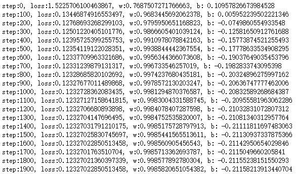
1.7 线性拟合
linear = LinearRegression()  # 线性回归
linear.fit(x.reshape(-1, 1), y)

plt.scatter(x, y)
x_test = np.linspace(0, 10, 20).reshape(-1, 1)
plt.plot(x_test, linear.coef_ * x_test + linear.intercept_, c='r')  # 画线
plt.plot(x_test, w.numpy() * x_test + b.numpy(), c='g', lw=10, alpha=0.5)  # 画线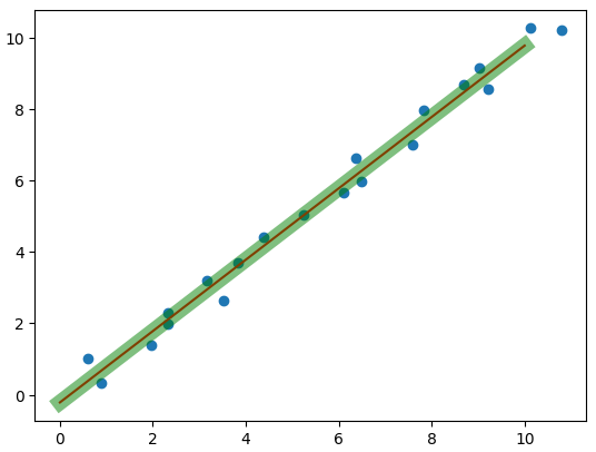
2. 使用TensorFlow实现 逻辑回归
实现逻辑回归的套路和实现线性回归差不多, 只不过逻辑回归的目标函数和损失函数不一样而已.
使用tensorflow实现逻辑斯蒂回归
- 找到预测函数 :
- 找到损失函数 : -(y_true * log(y_pred) + (1 - y_true)log(1 - y_pred))
- 梯度下降法求损失最小的时候的系数
2.1 导包
import  tensorflow as tf
from sklearn.datasets import make_blobs
import numpy as np
import matplotlib.pyplot as plt- 聚类数据生成器: make_blobs
2.2 描聚类数据点
data, target = make_blobs(centers = 2)
plt.scatter(data[:, 0] , data[:, 1], c = target)
x = data.copy()
y = target.copy()
print(x.shape, y.shape) # (100, 2) (100,) 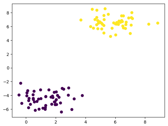
2.3 数据转换为张量 (tensor)
- 可以对目标值进行one_hot 编码: y = tf.one_hot(y, depth=2) # 可以添加, 进行优化
x = tf.constant(data, dtype = tf.float32)
y = tf.constant(target, dtype = tf.float32)
2.4 定义预测函数 (初始化w, b)
# 定义预测变量
W = tf.Variable(np.random.randn(2, 1) * 0.2, dtype = tf.float32)
B = tf.Variable(0., dtype = tf.float32)
2.5 定义目标函数
def sigmoid(x):
    linear = tf.matmul(x, W) + B
    return tf.nn.sigmoid(linear)
2.6 定义损失
# 定义损失
def cross_entropy_loss(y_true, y_pred):
    # y_pred 是概率,存在可能性是0, 需要进行截断
    y_pred = tf.reshape(y_pred, shape = [100])
    y_pred = tf.clip_by_value(y_pred, 1e-9, 1)
    return tf.reduce_mean(-(tf.multiply(y_true, tf.math.log(y_pred)) + tf.multiply((1 - y_pred),
                            tf.math.log(1 - y_pred))))
2.7 定义优化器
# 定义优化器
optimizer = tf.optimizers.SGD()

def run_optimization():
    with tf.GradientTape() as g:
        # 计算预测值
        pred = sigmoid(x)  # 结果为概率
        loss = cross_entropy_loss(y, pred)

    #计算梯度
    gradients = g.gradient(loss, [W, B])
    # 更新W, B
    optimizer.apply_gradients(zip(gradients, [W, B]))
2.8 定义准确率
- 准确率定义为二分类
# 计算准确率
def accuracy(y_true, y_pred):
    # 需要把概率转换为类别
    # 概率大于0.5 可以判断为正例
    y_pred = tf.reshape(y_pred, shape = [100])
    y_ = y_pred.numpy() > 0.5
    y_true = y_true.numpy()
    return (y_ == y_true).mean()
2.9 开始训练
# 定义训练过程
for i in range(5000):
    run_optimization()
    if i % 100 == 0:
        pred = sigmoid(x)
        acc = accuracy(y, pred)
        loss = cross_entropy_loss(y, pred)
        print(f'训练次数:{i}, 准确率: {acc}, 损失: {loss}')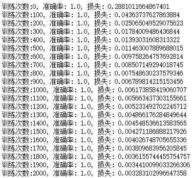


 458
458


 被折叠的 条评论
为什么被折叠?
被折叠的 条评论
为什么被折叠?
 到【灌水乐园】发言


