机器学习笔记(三)——模型评估及正则化

模型评估及正则化

误差计算

1. 对于线性回归模型，误差计算公式如下。

$$\text{err}(\theta )=\frac{1}{2m}\sum _{i=1}^m{\left(h_{\theta }\left(x^{(i)}\right)-y^{(i)}\right)}^2\text{\hspace{1em}(1)}$$

2. 对于逻辑回归模型，可以使用错误分类比率计算误差。

$$\begin{array}{r}\mathrm{err}\left(h_{\theta }(x),y\right)=\{\begin{array}{cc}& 1\text{ if }h(x)\ge 0.5\text{ and }y=0,\text{ or if }h(x)<0.5\text{ and }y=1\\ & 0\text{ Otherwise }\end{array}\end{array}\text{\hspace{1em}(2)}$$

$$\text{err}(\theta )=\frac{1}{m}\sum _{i=1}^m\mathrm{err}\left(h_{\theta }(x),y\right)\text{\hspace{1em}(3)}$$

模型选择

假设我们要在10个不同次数的二项式模型之间选择：
$$\begin{array}{rl}& h_{\theta }(x)={\theta }_0+{\theta }_{1}x\\ & h_{\theta }(x)={\theta }_0+{\theta }_{1}x+{\theta }_2{x}^2\\ & h_{\theta }(x)={\theta }_0+{\theta }_{1}x+\cdots +{\theta }_3{x}^3\\ & ⋮\\ & h_{\theta }(x)={\theta }_0+{\theta }_{1}x+\cdots +{\theta }_{10}{x}^{10}\end{array}\text{\hspace{1em}(4)}$$
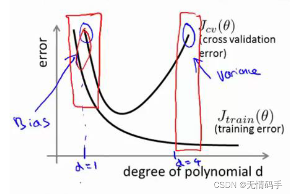
虽然多项式次数越高，训练集的误差越低，但在这同时该模型的泛化性下降，模型过拟合(方差)。

因此我们需要使用交叉验证集帮助选择模型。

首先我们要定义训练集、交叉验证集、测试集的误差。
$${\text{err}}_{\text{train }}(\theta )=\frac{1}{2m}\sum _{i=1}^m{\left(h_{\theta }\left(x^{(i)}\right)-y^{(i)}\right)}^2$$
$${\text{err}}_{cv}(\theta )=\frac{1}{2m_{cv}}\sum _{i=1}^{m_{cv}}{\left(h_{\theta }\left(x_{cv}^{(i)}\right)-y_{cv}^{(i)}\right)}^2\text{\hspace{1em}(5)}$$
$${\text{err}}_{\text{test }}(\theta )=\frac{1}{2m_{\text{test }}}\sum _{i=1}^{m_{\text{test }}}{\left(h_{\theta }\left(x_{\text{test }}^{(i)}\right)-y_{\text{test }}^{(i)}\right)}^2$$
选择方法：

1. 先用训练集去训练不同模型下的$minJ(\theta )$（这里的$J(\theta )$不同于$\text{err}(\theta )$，它是带正则化的）得到训练好的参数；
2. 用不同模型下训练得到的$\theta$去计算${\text{err}}_{cv}$，选择最小${\text{err}}_{cv}$对应的模型和参数作为我们将要使用的模型；
3. 计算${\text{err}}_{test}$。

方差和偏差

Bias和Variance分别从两个方面来描述我们学习到的模型与真实模型之间的差距。

Bias是用所有可能的训练数据集训练出的所有模型的输出的平均值与真实模型的输出值之间的差异。

Variance是不同的训练数据集训练出的模型输出值之间的差异。

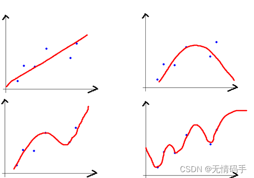
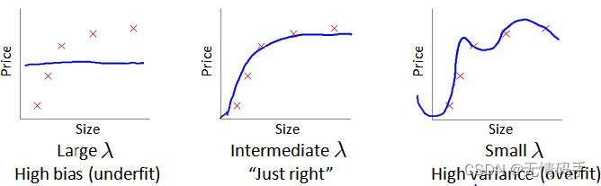
以上图为例：

1. 左上的模型偏差最大，右下的模型偏差最小；

2. 左上的模型方差最小，右下的模型方差最大。

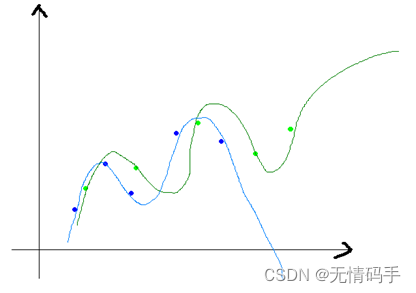
为了理解第二点，可以看下图。蓝色和绿色分别是同一个训练集上采样得到的两个训练子集，由于采取了复杂的算法去拟合，两个模型差异很大。如果是拿直线来拟合的话，显然差异不会这么大。

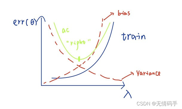
一般来说，偏差、方差和模型的复杂度之间的关系如下。因此在实际使用中，我们应该找到兼顾偏差和方差都小的模型。

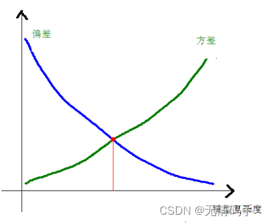
对于下图来说，当模型复杂度提升，方差增大，偏差减小。当模型复杂度减小，方差减小，偏差增大。

方差偏差和正则化

首先我想先介绍模型过拟合的原因，总结为如下两点：

1. 模型过于复杂;
2. 特征使用过多。

当特征使用过多时，我们可以选择减少使用的特征或者进行正则化。正则化程度越低，模型过拟合，方差越大，偏差越小。正则化程度越高，模型欠拟合，偏差越大，方差越小。如下图所示。

正则化系数确立

我们选择一系列的想要测试的$\lambda$值，通常是$ 0-10 $之间的呈现 2倍关系的值。如$0,0.01，0.02,0.04,0.08,0.16,...5.12,10.24$共12个。我们同样把数据分为训练集、交叉验证集和测试集。

选择$\lambda$的方法为：

1. 训练出不同$\lambda$下的模型；
2. 用不同的模型去计算交叉验证集下的误差；
3. 选择交叉验证集误差最小的模型；
4. 计算改模型下测试集的误差。

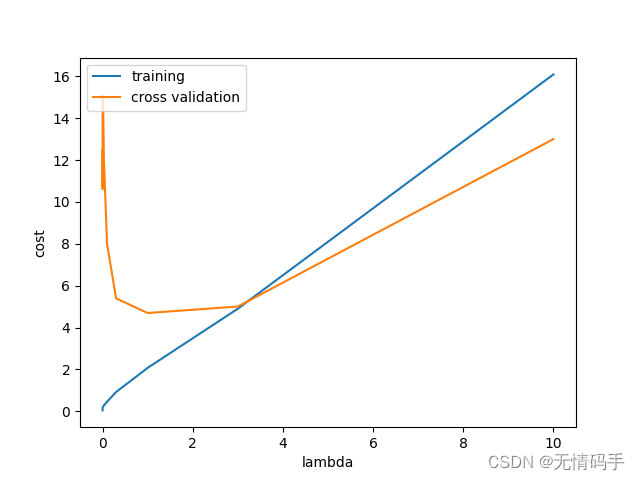
由下图可以看出，随着$\lambda$增大，训练集的误差在增大。交叉验证集的误差先减小后增大。图中还对应画出了方差与偏差的曲线。随着$\lambda$增大，方差逐渐减小，偏差逐渐增大。

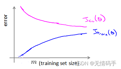
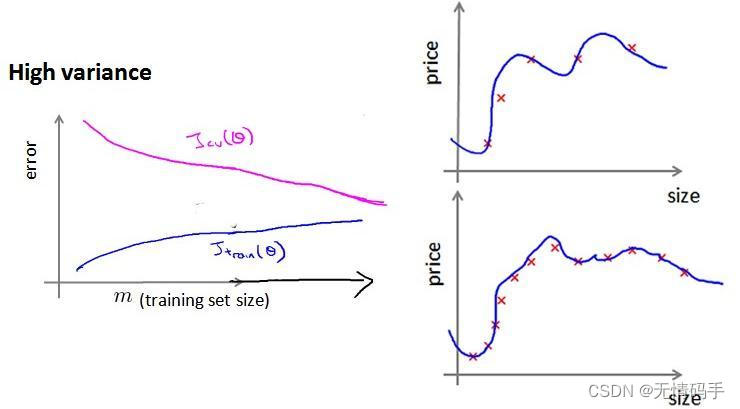
学习曲线

对于cv集来说，样本越少时，越不适应拟合的曲线，误差越大，样本越多时，越适应拟合的曲线，误差越小。

对于训练集来说，样本越少，拟合误差越小，样本越大，拟合误差越大。

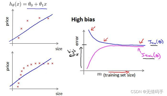
如下图所示，在高偏差/欠拟合的情况下，增加数据到训练集不一定有作用。也就是说，只要达到一定的训练样本，就已经得到了对应的拟合曲线，增加数据量后变化也不会太大。

如下图所示，对于高方差/过拟合的情况，增加数据到训练集可能可以提高算法的效果。

结论

1. 获得更多的训练实例——解决高方差
2. 尝试减少特征的数量——解决高方差
3. 尝试获得更多的特征——解决高偏差
4. 尝试增加多项式特征——解决高偏差
5. 尝试减少正则化程度$\lambda$——解决高偏差
6. 尝试增加正则化程度$\lambda$——解决高方差

代码

线性模型拟合数据

import numpy as np
import scipy.io as sio
import scipy.optimize as opt
import pandas as pd
import matplotlib.pyplot as plt

def load_data():
    #载入数据
    d = sio.loadmat('ex5data1.mat')
    return map(np.ravel, [d['X'], d['y'], d['Xval'], d['yval'], d['Xtest'], d['ytest']])

X, y, Xval, yval, Xtest, ytest = load_data()
print(X.shape,y.shape,Xval.shape,yval.shape,Xtest.shape,ytest.shape)
print(X[0])

处理数据格式。

#先把x转为(,1)的形式--->从1维转为2维
#从(12,)->(12,1) 再在第0位插入 1 按列插
X, Xval, Xtest = [np.insert(x.reshape(x.shape[0], 1), 0, np.ones(x.shape[0]), axis=1) for x in (X, Xval, Xtest)]
print(X[0])
print(X.shape,Xval.shape,Xtest.shape)

线性模型代价函数、梯度。

def cost(theta, X, y):
    m = X.shape[0]
    # tf.matmul(A,C)=np.dot(A,C)= A@C都属于叉乘，而tf.multiply(A,C)= A*C=A∙C属于点乘
    inner = X @ theta - y  # R(m*1)

    # 1*m @ m*1 = 1*1 in matrix multiplication
    square_sum = inner.T @ inner
    cost = square_sum / (2 * m)
    return cost

def gradient(theta, X, y):
    m = X.shape[0]
    #线性分类器的梯度
    inner = X.T @ (X @ theta - y)  # (m,n).T @ (m, 1) -> (n, 1)
    return inner / m

加正则化的梯度、加正则化的代价函数。梯度向量(矩阵)是给每个元素加对应参数本身的值做正则项。代价函数是把整个\theta的sum用做算正则项。

def regularized_gradient(theta, X, y, l=1):
    m = X.shape[0]

    regularized_term = theta.copy()  # same shape as theta
    regularized_term[0] = 0  # don't regularize intercept theta

    regularized_term = (l / m) * regularized_term
    # 针对于每个\theta计算梯度，直接把梯度的正则项加到梯度矩阵里
    return gradient(theta, X, y) + regularized_term

def regularized_cost(theta, X, y, l=1):
    m = X.shape[0]

    regularized_term = (l / (2 * m)) * np.power(theta[1:], 2).sum()

    return cost(theta, X, y) + regularized_term

线性回归。

def linear_regression_np(X, y, l=1):
    # init theta
    theta = np.ones(X.shape[1])

    # train it
    res = opt.minimize(fun=regularized_cost,
                       x0=theta,
                       args=(X, y, l),
                       method='TNC',
                       jac=regularized_gradient,
                       options={'disp': True})
    return res

theta = np.ones(X.shape[0])
final_theta = linear_regression_np(X, y, l=0).get('x')

b = final_theta[0] # intercept
m = final_theta[1] # slope

绘制散点图、连线图，并计算误差。

#区分 一个是scatter-->画散点 一个是 plot--两点之间画连线
plt.scatter(X[:,1], y, label="Training data")
plt.plot(X[:, 1], X[:, 1]*m + b, label="Prediction")
plt.legend(loc=2)
plt.show()

计算不同训练集m样本数训练得到模型的训练集和cv集的误差。

training_cost, cv_cost = [], []
m = X.shape[0]
for i in range(1, m + 1):
    #     print('i={}'.format(i))
    res = linear_regression_np(X[:i, :], y[:i], l=0)

    tc = regularized_cost(res.x, X[:i, :], y[:i], l=0)
    cv = regularized_cost(res.x, Xval, yval, l=0)
    #     print('tc={}, cv={}'.format(tc, cv))

    training_cost.append(tc)
    cv_cost.append(cv)

plt.plot(np.arange(1, m+1), training_cost, label='training cost')
plt.plot(np.arange(1, m+1), cv_cost, label='cv cost')
plt.legend(loc=1)
plt.show()

此模型欠拟合，因此我们使用多项式特征。

利用多项式特征训练模型

使用多项式特征，就是先把数据X变为$X^1$, …, $X^n$的形式。
原来的线性拟合只有 (1,x)截距和一个x值，现在的多项式回归是(1,$x^1$,$x^2$,…,$x^n$)，这里先要准备多项式回归数据。

def poly_features(x, power, as_ndarray=False):
    # 创建字典，key是f_i value是x^i
    data = {'f{}'.format(i): np.power(x, i) for i in range(1, power + 1)}
    # 转为pd.DataFrame,把每个f_i变成列向量
    df = pd.DataFrame(data)

    return df.as_matrix() if as_ndarray else df

def normalize_feature(df):
    """Applies function along input axis(default 0) of DataFrame."""
    # df的每一列(X_i)做标准化
    return df.apply(lambda column: (column - column.mean()) / column.std())

def prepare_poly_data(*args, power):
    """
    args: keep feeding in X, Xval, or Xtest
        will return in the same order
    """
    def prepare(x):
        # 先poly_features 变成 多列 x^n的形式，再标准化，再在第一列插入一列1 (行数代表样本数,列数是说多项式最高次数)
        # expand feature 扩展了x的列，维数
        df = poly_features(x, power=power)

        # normalization
        # 标准化后转为矩阵(即取出里面的值)
        ndarr = normalize_feature(df).values
        print(ndarr)

        # add intercept term
        # 在第一列插一列1
        return np.insert(ndarr, 0, np.ones(ndarr.shape[0]), axis=1)

    #可以输入多个变量，逐个变量进行prepare的操作
    return [prepare(x) for x in args]

加载数据，并初始化多项式数据。

X, y, Xval, yval, Xtest, ytest = load_data()
X_poly, Xval_poly, Xtest_poly= prepare_poly_data(X, Xval, Xtest, power=8)

定义学习曲线。

def plot_learning_curve(X, y, Xval, yval, l=0):
    training_cost, cv_cost = [], []
    m = X.shape[0]

    for i in range(1, m + 1):
        # regularization applies here for fitting parameters
        res = linear_regression_np(X[:i, :], y[:i], l=l)

        # remember, when you compute the cost here, you are computing
        # non-regularized cost. Regularization is used to fit parameters only
        tc = cost(res.x, X[:i, :], y[:i])
        cv = cost(res.x, Xval, yval)

        training_cost.append(tc)
        cv_cost.append(cv)

    plt.plot(np.arange(1, m + 1), training_cost, label='training cost')
    plt.plot(np.arange(1, m + 1), cv_cost, label='cv cost')
    plt.legend(loc=1)

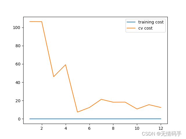
分别绘制$\lambda =0,1,20$情况下的学习曲线。

#没有正则化
plot_learning_curve(X_poly, y, Xval_poly, yval, l=0)
plt.show()

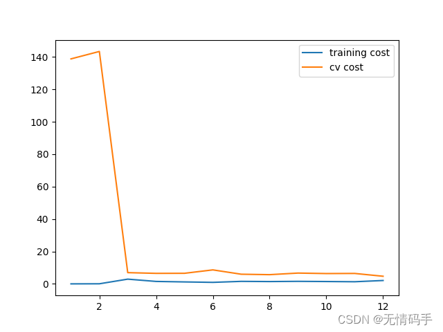
#\lambda = 1
plot_learning_curve(X_poly, y, Xval_poly, yval, l=1)
plt.show()

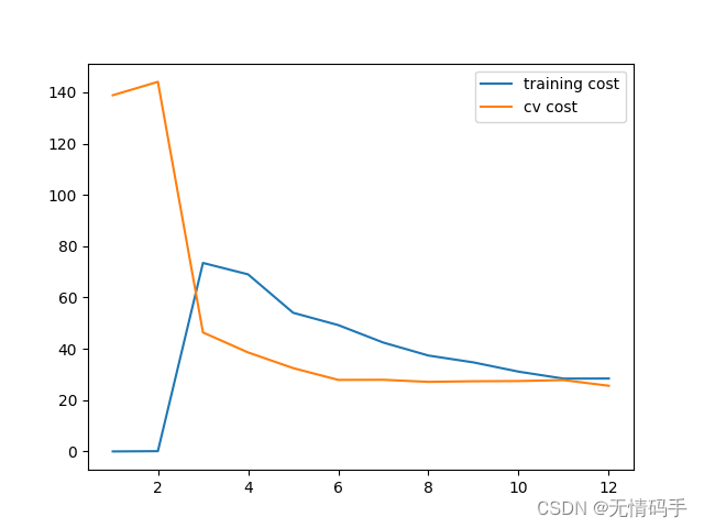
#\lambda = 20
plot_learning_curve(X_poly, y, Xval_poly, yval, l=20)
plt.show()

找到最佳$\lambda$。

# 找到最佳\lambda
l_candidate = [0, 0.001, 0.003, 0.01, 0.03, 0.1, 0.3, 1, 3, 10]
training_cost, cv_cost = [], []
for l in l_candidate:
    res = linear_regression_np(X_poly, y, l)

    tc = cost(res.x, X_poly, y)
    cv = cost(res.x, Xval_poly, yval)

    training_cost.append(tc)
    cv_cost.append(cv)
plt.plot(l_candidate, training_cost, label='training')
plt.plot(l_candidate, cv_cost, label='cross validation')
plt.legend(loc=2)

plt.xlabel('lambda')

plt.ylabel('cost')
plt.show()

得到最佳$\lambda$下的$\theta$，并计算${\text{err}}_{test}$。

l = l_candidate[np.argmin(cv_cost)]

theta = linear_regression_np(X_poly, y, l).x
print('test cost(l={}) = {}'.format(l, cost(theta, Xtest_poly, ytest)))

参考

(18 封私信 / 80 条消息) 偏差和方差有什么区别？ - 知乎 (zhihu.com)

偏差（Bias）与方差（Variance） - 知乎 (zhihu.com)