正则化(regularization)总结

一.为什么需要正则化?

简单来说，在使用神经网络时，为了增加模型的泛化能力，防止模型只在训练集上有效、在测试集上不够有效，我们使用正则化

正则化是为了防止过拟合， 进而增强泛化能力。用白话文转义，泛化误差（generalization error）= 测试误差（test error）。也可以说是为了使得训练数据训练的模型在测试集上的表现（或说性能 performance）好不好

二.正则化有哪几种常用方法？

常用的有$l_1-norm$、$l_2-norm$即在损失函数中添加惩罚项;还有例如$Droupout$方法。下面让我们来更仔细地看一下是怎么进行的

2.1 $l_1-norm$

$l_1-norm$也叫做lasso回归。
机器学习模型当中的参数，可形式化地组成参数向量，记为$\vec{w}$，为方便表示，我下面都记为大写字母W。不失一般性，以线性模型为例，模型可记为
$$F(x;W)=W^{T}x=\sum _{i=1}^n{w}_i\cdot x$$
为了进一步地偷懒，我们将$W^T$也叫做$W$。
现在我们来定义一个平方损失函数，其中W是模型的参数矩阵，x为模型的某个输入值，y为实际值，那么有损失函数
$$C=||Wx-y|{|}^2$$
所以有模型参数
$$W^{\ast }=arg\underset{C}{\min }||Wx-y|{|}^2$$
试想，假如我们使用某种方法使得cost降到最小，那么可想而知很容易便会产生过拟合(overfitting)。现在我们不希望这个cost降到最低，一个可行的方法是在损失函数公式中我们给它加入一个反向的干扰项，我们给它取个更专业的名字–惩罚项。
我们重新定义这个这个损失函数。$l_1-norm$方法在式子中加入了一个一次的惩罚项,用来描述模型的复杂程度
$$C=||Wx-y|{|}^2+\alpha ||W||$$
其中$\alpha$用来衡量惩罚项的重要程度。
使用这样的损失函数，便可以一定程度上防止产生过拟合了

2.2 $l_2-norm$

将惩罚项定位二次项，这样定义损失函数的方法我们称之为$l_2-norm$,也可以叫它Ridge回归（岭回归）。例如:
$$C=||Wx-y|{|}^2+\alpha ||W|{|}^2$$

2.3 Dropout正则化

L1、L2正则化是通过修改损失函数来实现的，而Dropout则是通过修改神经网络本身来实现的，它是在训练网络时用的一种技巧(trick)。
举例来说，假如现在我们有20个样本，但是定义了300个神经元，那么直接进行训练，由于神经元数量很多，所以模型的拟合效果会很好，也因此会很容易产生过拟合现象。现在我们每一次训练神经网络时，随机丢弃一部分神经元，下一次训练时，再随机丢掉一部分神经元，那么这样我们也可以有效降低过拟合效应。
下面是一个示例代码，来自莫烦py教程

import torch
import matplotlib.pyplot as plt

# torch.manual_seed(1)    # reproducible

N_SAMPLES = 20
N_HIDDEN = 300

# training data
x = torch.unsqueeze(torch.linspace(-1, 1, N_SAMPLES), 1)
y = x + 0.3*torch.normal(torch.zeros(N_SAMPLES, 1), torch.ones(N_SAMPLES, 1))

# test data
test_x = torch.unsqueeze(torch.linspace(-1, 1, N_SAMPLES), 1)
test_y = test_x + 0.3*torch.normal(torch.zeros(N_SAMPLES, 1), torch.ones(N_SAMPLES, 1))

# show data
plt.scatter(x.data.numpy(), y.data.numpy(), c='magenta', s=50, alpha=0.5, label='train')
plt.scatter(test_x.data.numpy(), test_y.data.numpy(), c='cyan', s=50, alpha=0.5, label='test')
plt.legend(loc='upper left')
plt.ylim((-2.5, 2.5))
plt.show()

net_overfitting = torch.nn.Sequential(
    torch.nn.Linear(1, N_HIDDEN),
    torch.nn.ReLU(),
    torch.nn.Linear(N_HIDDEN, N_HIDDEN),
    torch.nn.ReLU(),
    torch.nn.Linear(N_HIDDEN, 1),
)

net_dropped = torch.nn.Sequential(
    torch.nn.Linear(1, N_HIDDEN),
    torch.nn.Dropout(0.5),  # drop 50% of the neuron
    torch.nn.ReLU(),
    torch.nn.Linear(N_HIDDEN, N_HIDDEN),
    torch.nn.Dropout(0.5),  # drop 50% of the neuron
    torch.nn.ReLU(),
    torch.nn.Linear(N_HIDDEN, 1),
)

print(net_overfitting)  # net architecture
print(net_dropped)

optimizer_ofit = torch.optim.Adam(net_overfitting.parameters(), lr=0.01)
optimizer_drop = torch.optim.Adam(net_dropped.parameters(), lr=0.01)
loss_func = torch.nn.MSELoss()

plt.ion()   # something about plotting

for t in range(500):
    pred_ofit = net_overfitting(x)
    pred_drop = net_dropped(x)
    loss_ofit = loss_func(pred_ofit, y)
    loss_drop = loss_func(pred_drop, y)

    optimizer_ofit.zero_grad()
    optimizer_drop.zero_grad()  # 清空过往梯度，才能更顺利地进行再一次地计算梯度
    loss_ofit.backward()
    loss_drop.backward()  # backward通过反向传播计算当前梯度
    optimizer_ofit.step()  # step才更新网络参数
    optimizer_drop.step()

    if t % 10 == 0:
        # change to eval mode in order to fix drop out effect
        net_overfitting.eval()
        net_dropped.eval()  # parameters for dropout differ from train mode

        # plotting
        plt.cla()
        test_pred_ofit = net_overfitting(test_x)
        test_pred_drop = net_dropped(test_x)
        plt.scatter(x.data.numpy(), y.data.numpy(), c='magenta', s=50, alpha=0.3, label='train')
        plt.scatter(test_x.data.numpy(), test_y.data.numpy(), c='cyan', s=50, alpha=0.3, label='test')
        plt.plot(test_x.data.numpy(), test_pred_ofit.data.numpy(), 'r-', lw=3, label='overfitting')
        plt.plot(test_x.data.numpy(), test_pred_drop.data.numpy(), 'b--', lw=3, label='dropout(50%)')
        plt.text(0, -1.2, 'overfitting loss=%.4f' % loss_func(test_pred_ofit, test_y).data.numpy(), fontdict={'size': 20, 'color':  'red'})
        plt.text(0, -1.5, 'dropout loss=%.4f' % loss_func(test_pred_drop, test_y).data.numpy(), fontdict={'size': 20, 'color': 'blue'})
        plt.legend(loc='upper left'); plt.ylim((-2.5, 2.5));plt.pause(0.1)

        # change back to train mode
        net_overfitting.train()
        net_dropped.train()

plt.ioff()
plt.show()

结果：

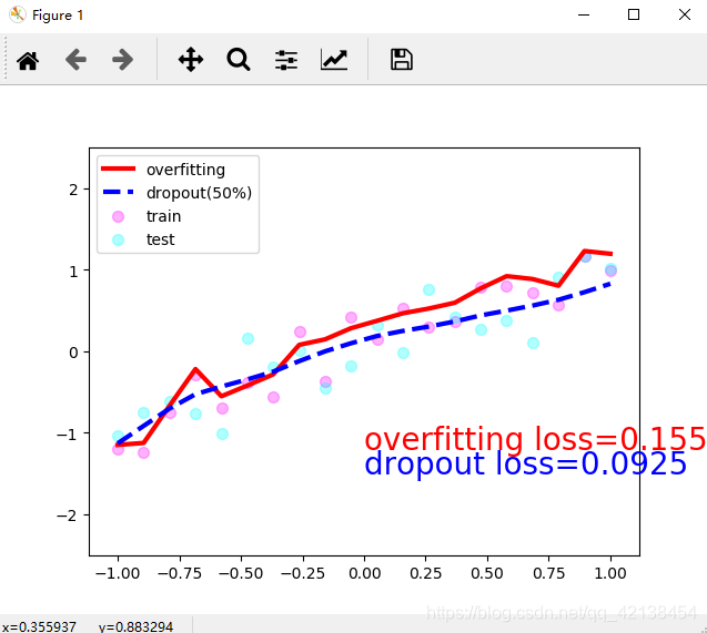
可以看到进行dropout后的网络在所有数据上的loss更小

总结一下我们应该怎么使用这种dropout技巧：

1. 定义网络时，在隐藏层中间使用torch.nn.Dropout(prop)
2. 神经网络有eval()和train()两种模式。计算预测值时记得切换到eval()模式，这种模式会关闭dropout；而在train()模式下，使用模型进行预测时仍然有部分神经元被dropout

2.4 增加训练集样本数量

这种方法自然也是可以削减过拟合的

参考

• 正则化理解
• L1与L2正则化
• 莫烦python