


文章目录
- 论文地址:https://papers.nips.cc/paper/2017/file/3f5ee243547dee91fbd053c1c4a845aa-Paper.pdf
- 源码:tensor2tensor
- 来源:NIPS, 2017
- 关键词:Sequecnce Modeling, Neural Machine Translation
1 前言
该论文针对序列转换(Sequence Transduction)问题中常见的弊端,提出使用Attention来完成Sequence Transduction,提出了新的网络结构 — Transformer。
2 问题定义
在Sequence Transduction领域中,通常是基于encoder-decoder形式的循环神经网络或CNN的。也存在一些模型使用注意力机制将encoder和decoder连接起来。该论文提出了一种完全基于注意力机制的新型网络 — Transformer,不需要RNN或CNN。
在对序列进行处理时,RNN通常沿着输入/输出序列的顺序进行计算,将序列中元素的位置与计算的步骤相对齐。这样的处理方式看似天然地保留了序列形式,但是使得计算只能串行进行,难以并行,而且对于长序列的计算还会带来内存容量限制的问题。虽然目前已经有一些相关的工作关于RNN的并行化,但是RNN串行计算的问题依然存在。
注意力机制已经成为了序列建模中不可或缺的一部分,在建模序列中依赖的时候能够不用考虑输入/输出中的距离。但是之前的工作都是用于起连接作用,本文则将encoder-decoder完全建立在注意力机制上来完成序列的建模问题。并在机器翻译任务中检测了Transformer的效果。
3 Transformer

3.1 Encoder and Decoder
Transformer的结构如上图所示,其中左边为 N N N个相同的layer堆叠起来的组成的encoder,右边为 N N N个相同的layer堆叠起来组成的decoder。组成encoder的layer由两部分组成:Multi-head Attention、Fully connected Feed Forward。组成encoder的layer由三部分组成:两个Multi-head Attention、Fully connected Feed Forward。以上的Multi-head Attention和Fully connected FFN都有残差连接和layer normalization。这样每一部分的输出都可以表示为: L a y e r N o r m ( x + S u b l a y e r ( x ) ) LayerNorm(x + Sublayer(x)) LayerNorm(x+Sublayer(x)),其中 S u b l a y e r Sublayer Sublayer就是Multi-head Attention或Fully connected FFN。
其实Encoder和Decoder都是由Multi-head Attention和Fully connected FFN组成的,但是二者在Self-Attention上有一些差别。Decoder修改了Self-Attention,是为了保证在预测 i i i处的输出时,只能依赖 i i i之前的输出,同时也是为了保持自回归(auto-regressive)的性质。
3.2 Attention
一个注意力函数可以描述为:将一个query与一系列的key-value对(pair)进行映射得到一个输出,其中的query、keys、values和输出均为向量。输出时values的加权求和,values对应的权是通过query与key计算得到的。

该论文中采用的是Scaled Dot-Product Attention,其计算过程如上图所示,写成公式为:
Attention
(
Q
,
K
,
V
)
=
softmax
(
Q
K
T
d
k
)
V
\operatorname{Attention}(Q, K, V)=\operatorname{softmax}\left(\frac{Q K^{T}}{\sqrt{d_{k}}}\right) V
Attention(Q,K,V)=softmax(dkQKT)V
有两种常用的attention函数:additive attention和dot-product attention。该论文中使用的是dot-product attention,但是略微不同,是Scaled后的dot-product attention。为什么要对dot-product 进行scaled呢?
当query、key的维度很大时,点积后的值可能会很大,可能会使softmax函数进入梯度很小的区域}。举个例子,加入q和k都是服从均值为0,方差为1的分布的随机变量,那么
q
⋅
k
=
∑
i
=
1
d
q
i
k
i
q \cdot k = \sum_{i=1}^{d} q_i k_i
q⋅k=∑i=1dqiki,结果的均值为0,但是方差为
d
d
d。
论文中使用了Multi-head Attention。从上图可以看出,在进行Multi-head Attention之前,先对Q、K、V进行了线性映射:
MultiHead
(
Q
,
K
,
V
)
=
Concat
(
head
1
,
…
,
head
h
)
W
O
where head
i
=
Attention
(
Q
W
i
Q
,
K
W
i
K
,
V
W
i
V
)
\begin{aligned} \operatorname{MultiHead}(Q, K, V) &=\text { Concat }\left(\text { head }_{1}, \ldots, \text { head }_{\mathrm{h}}\right) W^{O} \\ \quad \text { where head }_{\mathrm{i}} &=\text { Attention }\left(Q W_{i}^{Q}, K W_{i}^{K}, V W_{i}^{V}\right) \end{aligned}
MultiHead(Q,K,V) where head i= Concat ( head 1,…, head h)WO= Attention (QWiQ,KWiK,VWiV)
在Multi-Head Attention后就是Position-wise Feed-Forward Networks。从名字 — Position-wise也可以看出,Multi-head Attention的输出是逐个通过FFN的。在输入Attention函数之前,各个位置上的元素可以看作是独立的,不包含元素之间的依赖关系,经过Attention函数后,各个元素不仅包含了本身的含义还包含了与其他元素的依赖关系。所以不需要串行地通过FFN,FFN这一步操作是可以并行化的。
因为Transformer本身是不包含循环和卷积的,为了使模型利用序列中的顺序,论文中将\textbf{Positional Encoding}“加”到输入序列中的元素上。论文中使用的Positional-Encoding:
P
E
(
p
o
s
,
2
i
)
=
sin
(
p
o
s
/
1000
0
2
i
/
d
model
)
P
E
(
p
o
s
,
2
i
+
1
)
=
cos
(
p
o
s
/
1000
0
2
i
/
d
model
)
\begin{aligned} P E_{(p o s, 2 i)} &=\sin \left(p o s / 10000^{2 i / d_{\text {model }}}\right) \\ P E_{(p o s, 2 i+1)} &=\cos \left(p o s / 10000^{2 i / d_{\text {model }}}\right) \end{aligned}
PE(pos,2i)PE(pos,2i+1)=sin(pos/100002i/dmodel )=cos(pos/100002i/dmodel )
其中
p
o
s
,
i
pos,i
pos,i分别表示position和位置编码的维度。作者选用这样的位置编码的原因:使不同位置的元素能够通过相对位置更好地与当前元素建立关系,因为对于任意固定的
k
k
k,
P
E
p
o
s
+
k
PE_{pos+k}
PEpos+k可以表示为
P
E
p
o
s
PE_{pos}
PEpos的线性函数。
4 Why Self-Attention
Layer Type
Complexity per Layer
Sequential
Operations
Maximum Path Length
Self-Attention
O
(
n
2
⋅
d
)
O
(
1
)
O
(
1
)
Recurrent
O
(
n
⋅
d
2
)
O
(
n
)
O
(
n
)
Convolutional
O
(
k
⋅
n
⋅
d
2
)
O
(
1
)
O
(
log
k
(
n
)
)
Self-Attention (restricted)
O
(
r
⋅
n
⋅
d
)
O
(
1
)
O
(
n
/
r
)
\begin{array}{lccc} \hline \text { Layer Type } & \text { Complexity per Layer } & \begin{array}{c} \text { Sequential } \\ \text { Operations } \end{array} & \text { Maximum Path Length } \\ \hline \text { Self-Attention } & O\left(n^{2} \cdot d\right) & O(1) & O(1) \\ \text { Recurrent } & O\left(n \cdot d^{2}\right) & O(n) & O(n) \\ \text { Convolutional } & O\left(k \cdot n \cdot d^{2}\right) & O(1) & O\left(\log _{k}(n)\right) \\ \text { Self-Attention (restricted) } & O(r \cdot n \cdot d) & O(1) & O(n / r) \\ \hline \end{array}
Layer Type Self-Attention Recurrent Convolutional Self-Attention (restricted) Complexity per Layer O(n2⋅d)O(n⋅d2)O(k⋅n⋅d2)O(r⋅n⋅d) Sequential Operations O(1)O(n)O(1)O(1) Maximum Path Length O(1)O(n)O(logk(n))O(n/r)
与RNN/CNN相比,使用Self-Attention主要有三个原因:
- 计算复杂度
- 可并行的计算量
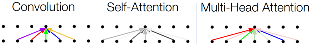
- 长范围依赖关系中的路径长度(注意:长范围的依赖不一定代表距离远)。路径越短,越容易学习到长范围的依赖。Self-Attention中将每个位置的元素都直接与其他位置的元素相连。从Attention的输入和输出来看,CNN和Attention之间是有一定相似性的,如下图(原图见nlp-stanford/Tensor2Tensor Transformers New Deep Models for NLP)所示。Multi-head能够捕捉多种关系。在较长的输入序列下,可以选择restricted的self-attention,即每个位置只考虑周围固定数量的邻居
三者的比较见上表。
5 方法的优势
- 提出了完全基于Attention机制的序列建模
- 基于Attention的Transformer中的大量操作都是可以并行的,大大降低计算的时间
- 对长范围依赖关系的建模
Attention参考资料
- The Annotated Transformer — Harvard Transformer tutorial
- Visualizing A Neural Machine Translation Model (Mechanics of Seq2seq Models With Attention)
- The Illustrated Transformer(力荐)
欢迎访问我的个人博客~~~
以及我的公众号【一起学AI】


 1万+
1万+


 被折叠的 条评论
为什么被折叠?
被折叠的 条评论
为什么被折叠?
 到【灌水乐园】发言


