Python | NumPy | 不完全总结

本文对 NumPy 进行不完全总结 ¹。

Last Modified: 2024 / 02 / 14

---

---

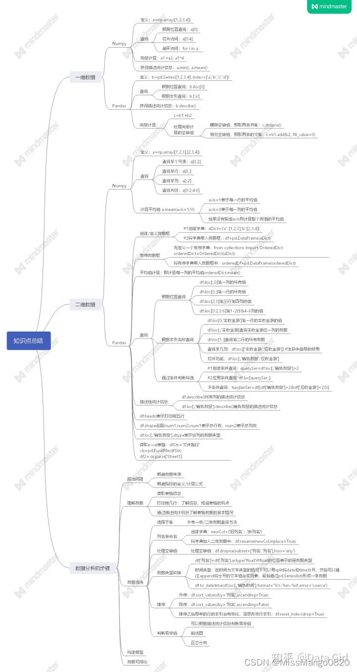
总览

Numpy与Pandas比较

下面的知识点总结图参考此处 [^numpy大法]

广播机制

在 Numpy 中当数组进行运算时，如果两个数组的形状相同，那么两个数组相加就是两个数组的对应位相加，这是要求维数相加，并且各维度的长度相同。比如：

data1 = np.arange(9,dtype=np.int32).reshape(3,3) 
# [[0 1 2]
#  [3 4 5]
#  [6 7 8]]

data2 = np.ones((3,3),dtype=np.int32)  
# [[1 1 1]
#  [1 1 1]
#  [1 1 1]]

data = data1 + data2
# [[1 2 3]
#  [4 5 6]
#  [7 8 9]]

当运算中两个数组的形状不同使时，numpy将会自动触发广播机制，那什么是广播机制呢？

复习下数学知识，在线性代数中我们曾经学到过如下规则：

• a1 = 3 ，a2 = 4，a1，a2 是 0 维张量，即标量。
  a1 与 a2 之间可以进行加减乘除
• b1，b2 是 1 维张量，即向量。
  b1 与 b2 可以进行逐元素的加减乘除运算
  
• c1，c2 是如下所示的 2 维张量，即矩阵。
  c1 与 c2 之间可以进行逐元素的加减乘除以及矩阵相乘运算 (矩阵相乘必须满足维度的对应关系)，而 a 与 b ，或者 b 与 c 之间不能进行逐元素的加减乘除运算，原因是他们的维度不匹配。而这种在数学方面的不可能在 NumPy 中，就可以通过广播完成这项操作。
  
  
  

比如：

data1 = np.arange(9,dtype=np.int32).reshape(3,3)
  
# [[0 1 2]
#  [3 4 5]
#  [6 7 8]]

print(data1+1)

# 此时data1是3行3列的矩阵，跟一个1进行运算，能否成功呢？在Numpy中这时ok的，data1中的每个元素都会跟1相加而得到一个新的矩阵，这就是广播机制。
# [[1 2 3]
#  [4 5 6]
#  [7 8 9]]

如果是跟一个 3 行 1 列的进行加法呢？

data2 = np.array([[1],[2],[3]])

# [[1]
#  [2]
#  [3]]

print(data1+data2)
# [[ 1  2  3]
#  [ 5  6  7]
#  [ 9 10 11]]

如果是跟一个 2 行 3 列的数据进行加法运算呢？

data3 = np.array([[1,2,3],[1,1,1]])
# [[1 2 3]
#  [1 1 1]]

print(data1+data3)
---------------------------------------------------------------------------
ValueError                                Traceback (most recent call last)
 in----> 1 print(data1+data2)

ValueError: operands could not be broadcast together with shapes (3,3) (2,3) 

报错的原因是什么呢？我们一起来看一张图：

所以广播的规则是：

1. 形状相同的广播；
2. 相同维度，但其中某一个或多个维度长度为 1 的广播；
3. 如果是标量的话，会广播整个数组上；

---

基本操作

Numpy 中 ndarray 对象是类似列表的，但是也有区别 ²，比如：

• 数组对象内的元素类型必须相同
• 数组大小不可修改

说明对ndarray的使用方法时，若无特殊举例，即以以下数组为例进行说明:

import numpy as np
arr = np.array([[7, 4, 3, 3], [7, 4, 3, 3], [4, 8, 3, 3], [1, 6, 3, 3]])
# [[7 4 3 3]
#  [7 4 3 3]
#  [4 8 3 3]
#  [1 6 3 3]]
# ⬆️ shape (4, 4)

属性

方法	含义
ndarray.shape	多維陣列的大小（形狀） 在示例中， arr.shape # (4, 4)
ndarray.ndim	多維陣列的維度 在示例中， arr.ndim # 2
ndarray.itemsize	陣列當中元素的大小（佔幾個 byte） 在示例中, arr.itemsize # 4
ndarray.nbytes	整個陣列所有元素的大小總計 在示例中， arr.nbytes # 64
ndarray.T	轉置矩陣，只能在維度 <= 2 的時候使用，與 self.transpose() 效果相同 arr.T #[[7 7 4 1] # [4 4 8 6] # [3 3 3 3] # [3 3 3 3]]
ndarray.flat	把陣列扁平化輸出

格式转换

此处以以下数组为例进行说明:

import numpy as np
arr = np.array([['a', 'b', 'c', 'd'], ['e', 'f', 'g', 'h'], ['i', 'j', 'k', 'l'], ['m', 'n', 'o', 'p']])
# [['a' 'b' 'c' 'd']
#  ['e' 'f' 'g' 'h']
#  ['i' 'j' 'k' 'l']
#  ['m' 'n' 'o' 'p']]
# ⬆️ shape (4, 4)

方法	含义
ndarray.item	類似 List 的 Index，把 Array 扁平化取得某 Index 的 value 在示例中， arr.item(15) # P
ndarray.tolist	把 NumPy.ndarray 輸出成 Python 原生 List 型態 在示例中， arr.tolist() # [['a', 'b', 'c', 'd'], ['e', 'f', 'g', 'h'], ['i', 'j', 'k', 'l'], ['m', 'n', 'o', 'p']]
ndarray.itemset	把 ndarray 中的某個值（純量）改掉 具体用法可参照此处 在示例中， arr.itemset((3, 3), 7) # [['a' 'b' 'c' 'd'] # ['e' 'f' 'g' 'h'] # ['i' 'j' 'k' 'l'] # ['m' 'n' 'o' '7']]

维度操作

方法	含义
ndarray.reshape(shape)	把同樣的資料以不同的 shape 輸出（array 的 total size 要相同） 在示例中， arr.reshape(2, 8) # [['a' 'b' 'c' 'd' 'e' 'f' 'g' 'h'] # ['i' 'j' 'k' 'l' 'm' 'n' 'o' 'p']] # ⬆️ shape (2, 8) arr.reshape(-1) # ['a' 'b' 'c' 'd' 'e' 'f' 'g' 'h' 'i' 'j' 'k' 'l' 'm' 'n' 'o' 'p'] # ⬆️ shape (16,)
ndarray.resize(shape)	重新定義陣列的大小 在示例中， arr.resize((2, 8)) # [['a' 'b' 'c' 'd' 'e' 'f' 'g' 'h'] # ['i' 'j' 'k' 'l' 'm' 'n' 'o' 'p']] # ⬆️ shape (2, 8)
ndarray.flatten()	把多維陣列收合成一維陣列（扁平化＆有原数据的副本） arr.flatten() # ['a' 'e' 'i' 'm' 'b' 'f' 'j' 'n' 'c' 'g' 'k' 'o' 'd' 'h' 'l' 'p'] # ⬆️ shape (16,)
ndarray.ravel()	回傳扁平化的陣列（无源数据的副本） 在示例中， arr.ravel() # ['a' 'b' 'c' 'd' 'e' 'f' 'g' 'h' 'i' 'j' 'k' 'l' 'm' 'n' 'o' 'p'] # ⬆️ shape (16,)

项目选择与操作

方法	含义
ndarray.take(indices)	根據輸入索引值來得到指定陣列 在示例中， arr.take(11) # l
ndarray.put(indices, values)	根據索引值改變陣列 value 在示例中， arr.put(11, 5) # [['a' 'b' 'c' 'd'] # ['e' 'f' 'g' 'h'] # ['i' 'j' 'k' '5'] # ['m' 'n' 'o' 'p']] # ⬆️ shape (4, 4)
ndarray.repeat(times)	重複陣列的值（類似擴張） 在示例中， arr.repeat(2) # ['a' 'a' 'b' 'b' 'c' 'c' 'd' 'd' 'e' 'e' 'f' 'f' 'g' 'g' 'h' 'h' 'i' 'i' 'j' 'j' 'k' 'k' 'l' 'l' 'm' 'm' 'n' 'n' 'o' 'o' 'p' 'p'] # ⬆️ shape (32,)
ndarray.sort()	把陣列當中的元素排序 在此处的示例中， arr = np.array([['o', 'n', 'm', 'p'], ['h', 'g', 'f', 'e'], ['k', 'i', 'j', 'l'], ['a', 'd', 'c', 'b']]) # [['o' 'n' 'm' 'p'] # ['h' 'g' 'f' 'e'] # ['k' 'i' 'j' 'l'] # ['a' 'd' 'c' 'b']] # ⬆️ shape (4, 4) arr.sort(axis=1) # [['m' 'n' 'o' 'p'] # ['e' 'f' 'g' 'h'] # ['i' 'j' 'k' 'l'] # ['a' 'b' 'c' 'd']] # ⬆️ shape (4, 4) arr.sort(axis=0) # [['a' 'b' 'c' 'd'] # ['e' 'f' 'g' 'h'] # ['i' 'j' 'k' 'l'] # ['m' 'n' 'o' 'p']] # ⬆️ shape (4, 4)
ndarray.sum()	加總多維陣列（可指定加總的維度根據） 在此处的示例中， arr = np.array([[7, 4, 3, 3], [4, 8, 3, 3]]) # [7 4 3 3] # [4 8 3 3] # ⬆️ shape (2, 4) arr.sum(axis=0) # [11 12 6 6] # ⬆️ shape (1, 4)

实用模块

方法	含义
np.squeeze(array)	去掉array的单维维度，可参照这里 ，以及这里 在此处示例中， arr = np.array([[['a', 'b']], [['c', 'd']], [['e', 'f']], [['g', 'h']]]) # [[['a' 'b']] # # [['c' 'd']] # # [['e' 'f']] # # [['g' 'h']]] # ⬆️ shape (4, 1, 2) np.squeeze(arr, axis=1)) # [['a' 'b'] # ['c' 'd'] # ['e' 'f'] # ['g' 'h']] # ⬆️ shape (4, 2)
np.maximin(x, y)	比较两个值大小 在此处示例中, np.maximin([3, 3], [7, 4]) # [7 4]

---

数据生成与复制、重复

生成

一维数组

单一数列

方法	含义
np.arange()	np.arange(10) # [0 1 2 3 4 5 6 7 8 9] # ⬆️ shape (1, 10) np.arange(3, 7) # [3 4 5 6] # ⬆️ shape (1, 4) np.arange(2, 8, 2) # [2 4 6] # ⬆️ shape (1, 3)
np.array(np.arange())	np.array(np.arange(10)) # [0 1 2 3 4 5 6 7 8 9] # ⬆️ shape (1, 10) np.array([10]) # [10] # ⬆️ shape (1,) np.array(10) # 10 # ⬆️ shape ()
np.linspace()	用于创建指定数量等间隔的序列，实际生成一个等差数列。 np.linspace(2.0, 8.0, num=4) [2. 4. 6. 8.] # ⬆️ shape (1, 4) ⬆️ 在[2.0， 8.0]的范围里，生成一个含有4个数字的一维数组
np.logspace()	用于生成等比数列。

矩阵

方法	含义
np.arange().reshape()	np.arange(10).reshape(2, 5) # [[0 1 2 3 4] # [5 6 7 8 9]] # ⬆️ shape (2, 5)
np.ones(shape)	构造全1矩阵 np.ones(3, 4) # [[1. 1. 1.] # [1. 1. 1.] # [1. 1. 1.] # [1. 1. 1.]] # ⬆️ shape (3, 4)
np.zeros(shape)	构造全0矩阵 np.zeros(3,4) # [[0. 0. 0.] # [0. 0. 0.] # [0. 0. 0.] # [0. 0. 0.]] # ⬆️ shape (3, 4)
np.eye()	构造对角单位矩阵 np.eye(4) # [[1. 0. 0. 0.] # [0. 1. 0. 0.] # [0. 0. 1. 0.] # [0. 0. 0. 1.]] # ⬆️ shape (4, 4)
np.empty(shape)	构造全空矩阵（实际有值） np.empty(shape=(2, 2)) # [[-3.10503618e+231 1.28822984e-231] # [ 9.88131292e-324 2.78134232e-309]] # ⬆️ shape (2, 2)

复制 / 重复

以以下数组为例，对复制/重复的方式 / 方法进行说明:

arr = np.array([[7, 4], [4, 8]])

复制

repeat，对数组中的元素进行连续重复复制。用法有2种。

方法	含义
numpy.repeat(a, repeats, axis=None)	np.repeat(arr, repeats=3, axis=1) # [[7 7 7 4 4 4] # [4 4 4 8 8 8]] # ⬆️ shape (2, 6) np.repeat(arr,repeats=3, axis=1) # [[7 4] # [7 4] # [7 4] # [4 8] # [4 8] # [4 8]] # ⬆️ shape (6, 2)
a.repeats(repeats, axis=None)	arr.repeat(repeats=3, axis=0) # [[7 4] # [7 4] # [7 4] # [4 8] # [4 8] # [4 8]] # ⬆️ shape (6, 2) arr.repeat(repeats=3, axis=1) # [[7 7 7 4 4 4] # [4 4 4 8 8 8]] # ⬆️ shape (2, 6)

重复

tile, 对整个数组进行复制、拼接

方法	含义
np.tile(A, reps)	a为数组，reps为重复的次数 np.tile(arr, reps=2) # [[7 4 7 4] # [4 8 4 8]] # ⬆️ shape (2, 4) np.tile(arr, (3, 2)) # [[7 4 7 4] # [4 8 4 8] # [7 4 7 4] # [4 8 4 8] # [7 4 7 4] # [4 8 4 8]] # ⬆️ shape (6, 4)

---

属性与统计、运算

矩阵属性

以下面这个数组为例对如何获取矩阵的属性进行说明：

arr = np.array([[['nan', 1], [8, '5'], ['4', 'nan']], [[5, 12], [3, 18], ['nan', 1]]], dtype=float)
# [[[nan  1.]
#   [ 8.  5.]
#   [ 4. nan]]
# 
#  [[ 5. 12.]
#   [ 3. 18.]
#   [nan  1.]]]
# ⬆️ shape (2, 3, 2)

方法	含义
arr.shape	矩阵横纵维度 arr.shape # (2, 3, 2)
arr.ndim	矩阵维度 arr.ndim # 3
arr.size	元素总数 arr.size # 12
arr.dtype	返回数组的数据类型 arr.dtype # float64
np.isnan(arr)	用于测试元素是否为NaN（非数字）。 isnan（）函数包含两个参数，其中一个是可选的。我们还可以传递数组，以检查数组中存在的项是否属于NaN类。如果为NaN，则该方法返回True，否则返回False。因此，isnan（）函数返回布尔值。 np.isnan(arr) # [[[ True False] # [False False] # [False True]] # # [[False False] # [False False] # [ True False]]] # ⬆️ shape (2, 3, 2)
np.where(np.isnan(arr), value, arr)	填充缺失值为目标值 np.where(np.isnan(arr), 0, arr) # [[[ 0. 1.] # [ 8. 5.] # [ 4. 0.]] # # [[ 5. 12.] # [ 3. 18.] # [ 0. 1.]]] # ⬆️ shape (2, 3, 2)
arr[arr<4]=0	arr数组中符合arr<4的数据被赋值为0 # [[[nan 0.] # [ 8. 5.] # [ 4. nan]] # # [[ 5. 12.] # [ 0. 18.] # [nan 0.]]] # ⬆️ shape (2, 3, 2)

数组拉直

以下面这个数组为例对如何拉直矩阵进行说明：

arr = np.array([[['nan', 1], [8, '5'], ['4', 'nan']], [[5, 12], [3, 18], ['nan', 1]]], dtype=float)
# [[[nan  1.]
#   [ 8.  5.]
#   [ 4. nan]]
# 
#  [[ 5. 12.]
#   [ 3. 18.]
#   [nan  1.]]]
# ⬆️ shape (2, 3, 2)

方法	含义
arr.ravel()	多维数组降为一维数组。 生成的是原数组的视图，无需占有内存空间，但视图的改变会影响到原数组的变化。 arr.ravel() # [nan 1. 8. 5. 4. nan 5. 12. 3. 18. nan 1.] # ⬆️ shape (12,) arrF[:3] = 1000 # [1000. 1000. 1000. 5. 4. nan 5. 12. 3. 18. nan 1.] # ⬆️ shape (12,) arr # [[[1000. 1000.] # [1000. 5.] # [ 4. nan]] # # [[ 5. 12.] # [ 3. 18.] # [ nan 1.]]] # ⬆️ shape (2, 3, 2)
arr.flatten()	多维数组降为一维数组 返回的是真实值，其值的改变并不会影响原数组的更改。 arr.flatten() # [nan 1. 8. 5. 4. nan 5. 12. 3. 18. nan 1.] # ⬆️ shape (12,) arrF[:3] = 1000 # [1000. 1000. 1000. 5. 4. nan 5. 12. 3. 18. nan 1.] # ⬆️ shape (12,) arr # [[[nan 1.] # [ 8. 5.] # [ 4. nan]] # # [[ 5. 12.] # [ 3. 18.] # [nan 1.]]] # ⬆️ shape (2, 3, 2)

矩阵运算

以以下3个维度不同的数组为例，对矩阵运算进行说明：

arrA = np.array(np.arange(1, 5)).reshape(2, 2)
# [[1 2]
# [3 4]]
# ⬆️ shape (2, 2)

arrB = np.array(np.arange(1, 3)).reshape(1, 2)
# [[1 2]]
# ⬆️ shape (1, 2)

arrC = np.array(np.arange(1, 9)).reshape(4, 2)
# [[1 2]
# [3 4]
# [5 6]
# [7 8]]
# ⬆️ shape (4, 2)

乘积

方法	含义
arr*arr	矩阵相乘: 1.两个arr的shape相同 2.两个arr的维度相同，其中一个维度上两个arr的shape相同且另一个维度上其中一个arr的shape应为1 <1.> arrA*arrA # [[ 1 4] # [ 9 16]] # ⬆️ shape (2, 2) np.prod(arr)) # 24 <2.> <2.1.> arrA*arrB # [[1 4] # [3 8]] # ⬆️ shape (2, 2) arrB*arrC # [[ 1 4] # [ 3 8] # [ 5 12] # [ 7 16]] # ⬆️ shape ((4, 2)) <2.2.> arrA*arrC ValueError: operands could not be broadcast together with shapes (2,2) (4,2)

相加

方法	含义
arr1+arr2	矩阵相加: 1.两个arr的shape相同 2.两个arr的维度相同，其中一个维度上两个arr的shape相同且另一个维度上其中一个arr的shape应为1 <2.> <2.1.> arrA+arrB # [[2 4] # [4 6]] # ⬆️ shape (2, 2) arrB+arrC # [[ 2 4] # [ 4 6] # [ 6 8] # [ 8 10]] # ⬆️ shape (4, 2) <2.2> arrA+arrC ValueError: operands could not be broadcast together with shapes (2,2) (4,2)

相减

相减 与 相加 同理。

示例

1.

对数组中的所有元素减去相同的数字 ³：

arrA - 3
# [[-2 -1]
#  [ 0  1]]

arrC - 2
# [[-1  0]
#  [ 1  2]
#  [ 3  4]
#  [ 5  6]]

矩阵运用函数

以以下2个维度不同的数组中任意一个为例，对矩阵运用函数进行说明：

arr2 = np.array((np.arange(1, 9))).reshape(2, 4)
# [[1 2 3 4]
#  [5 6 7 8]]
# ⬆️ shape (2, 4)

arr3 = np.array((np.arange(1, 13)).reshape(2, 2, 3))
# [[[ 1  2  3]
#   [ 4  5  6]]
#
#  [[ 7  8  9]
#   [10 11 12]]]
# ⬆️ shape (2, 2, 3)

乘积

方法	含义
np.prod()	矩阵内所有元素的积 <1.> np.prod(arr2) # 40320 <2.> np.prod(arr3) # 479001600
np.cumprod(a, axis)	累计积 <1> np.cumprod(a=arr2, axis=0) # [[ 1 2 3 4] # [ 5 12 2`1 32]] np.cumprod(a=arr2, axis=1) # [[ 1 2 6 24] # [ 5 30 210 1680]] <2> np.cumprod(a=arr3, axis=0) # [[[ 1 2 3] # [ 4 5 6]] # [[ 7 16 27] # [40 55 72]]] np.cumprod(a=arr3, axis=1) # [[[ 1 2 3] # [ 4 10 18]] # [[ 7 8 9] # [ 70 88 108]]]

示例

np.prod

np.prod([arr3, arr3], axis=0)
# [[[  1   4   9]
#   [ 16  25  36]]
#
#  [[ 49  64  81]
#   [100 121 144]]]
# ⬆️ shape (2, 2, 3)

np.prod([arr3, arr3], axis=1)
# [[[ 7 16 27]
#   [40 55 72]]
#
#  [[ 7 16 27]
#   [40 55 72]]]
# ⬆️ shape (2, 2, 3

np.cumprodu

相加

方法	含义
sum(arr)	返回沿最低维轴的加和值 <1.> sum(arr2) # [ 6 8 10 12] # ⬆️ shape (4,) <2.> sum(arr3) # [[ 8 10 12] # [14 16 18]] # ⬆️ shape (2, 3)
arr.sum(axis) / np.sum(a, axis)	返回的是一个矩阵总和 <1.> arr2.sum() # 36 arr2.sum(axis=0) # [ 6 8 10 12] # ⬆️ shape (4,) arr2.sum(axis=1) # [10 26] # ⬆️ shape (2,) <2.> arr3.sum() # 78 arr3.sum(axis=0) # [[ 8 10 12] # [14 16 18]] # ⬆️ shape (2, 3) arr3.sum(axis=1) # [[ 5 7 9] # [17 19 21]] # ⬆️ shape (2, 3)
arr.cumsum(axis)	返回沿低维轴的累计加和 <1.> arr2.cumsum() # [ 1 3 6 10 15 21 28 36] arr2.cumsum(axis=0) # [[ 1 2 3 4] # [ 6 8 10 12]] ⬆️ shape (2, 4) arr2.cumsum(axis=1) # [[ 1 3 6 10] # [ 5 11 18 26]] # ⬆️ shape (2, 4) <2.> arr3.cumsum() # [ 1 3 6 10 15 21 28 36 45 55 66 78] arr3.cumsum(axis=0) # [[[ 1 2 3] # [ 4 5 6]] # # [[ 8 10 12] # [14 16 18]]] # shape (2, 2, 3) arr3.cumsum(axis=1) # [[[ 1 2 3] # [ 5 7 9]] # # [[ 7 8 9] # [17 19 21]]] # ⬆️ shape (2, 2, 3)

平均值

方法	含义
arr.mean()	获得矩阵中元素的平均值，同样地，可以获得行或列的平均值。 <1.> arr2.mean() # 4.5 arr2.mean(axis=0) # [3. 4. 5. 6.] # ⬆️ shape (4,) arr2.mean(axis=1) # [2.5 6.5] # ⬆️ shape (2,) <2.> arr3.mean() # (2,) arr3.mean(axis=0) # [[4. 5. 6.] # [7. 8. 9.]] # ⬆️ shape (2, 3) arr3.mean(axis=1) # [[ 2.5 3.5 4.5] # [ 8.5 9.5 10.5]] # ⬆️ shape (2, 3)
np.mean(a, axis)	同⬆️

极值

方法	含义
arr.max()	获得整个矩阵、行或列的最大值 <1.> arr2.max() # 8 arr2.max(axis=0) # [5 6 7 8] # ⬆️ shape (4,) arr2.max(axis=1) # [4 8] # ⬆️ shape (2,) <2.> arr3.max() # 12 arr3.max(axis=0) # [[ 7 8 9] # [10 11 12]] # ⬆️ shape (2, 3) arr3.max(axis=1) # [[ 4 5 6] # [10 11 12]] # ⬆️ shape (2, 3)
arr.argmax(axis)	获得最大值元素所在的位置 <1.> arr2.argmax() # 7 arr2.argmax(axis=0) # [1 1 1 1] # ⬆️ shape (4,) arr2.argmax(axis=1) # [3 3] # ⬆️ shape [3 3] <2.> arr3.argmax() # 11 arr3.argmax(axis=0) # [[1 1 1] # [1 1 1]] # ⬆️ (2, 3) arr3.argmax(axis=1) # [[1 1 1] # [1 1 1]] # ⬆️ (2, 3)
arr.min()	获得整个矩阵、行或列的最小值 <1.> arr2.min() #1 arr2.min(axis=0) # [5 6 7 8] # ⬆️ shape (4,) arr2.min(axis=1) # [1 5] # ⬆️ shape (2,) <2.> arr3.min() # 1 arr3.min(axis=0) # [[[1 2 3] # [4 5 6]] # ⬆️ shape (2, 3) arr3.min(axis=1) # [[1 2 3] # [7 8 9]] # ⬆️ shape (3, 2)
arr.argmin(axis)	<1.> arr2.argmin() # 0 arr2.argmin(axis=0) [0 0 0 0] # ⬆️ shape (4,) arr2.argmin(axis=1) # [0 0] # ⬆️ shape (2,) <2.> arr3.argmin() # 0 arr3.argmin(axis=0) # [[0 0 0] # [0 0 0]] # ⬆️ shape (2, 3) arr3.argmin(axis=1) # [[0 0 0] # [0 0 0]] # ⬆️ shape (2, 3)

三角函数

方法	含义
np.sin(a)	对矩阵a中每个元素取正弦,sin(x)
np.cos(a)	对矩阵a中每个元素取余弦,cos(x)
np.tan(a)	对矩阵a中每个元素取正切,tan(x)
np.arcsin(a)	对矩阵a中每个元素取反正弦,arcsin(x)
np.arccos(a)	对矩阵a中每个元素取反余弦,arccos(x)
np.arctan(a)	对矩阵a中每个元素取反正切,arctan(x)

指数

方法	含义
np.exp(a)	对矩阵a中每个元素取指数函数,ex

根号

方法	含义
np.sqrt(a)	对矩阵a中每个元素开根号√x

方差

方法	含义
np.var(a, axis )	方差

标准差

方法	含义
np.std(a, axis)	标准差

偏度、峰度

---

导出及导入和格式转换

除非有特殊说明，否则以下面的数组为示例，对导出及导入和格式转换的内容进行说明：

arr = np.array((np.arange(1, 17))).reshape(2, 2, 4)
'''
[[[ 1  2  3  4]
  [ 5  6  7  8]]

 [[ 9 10 11 12]
  [13 14 15 16]]]

# ndim, 3
# shape, (2, 2, 4)
# type(arr), <class 'numpy.ndarray'>
# arr.dtype, int64
'''

导出及导入

此处以下面的示例为例介绍导出、导入的几种方法 ⁴，

arr = np.arange(24).reshape(3, 2, 4)
# [[[ 0  1  2  3]
#   [ 4  5  6  7]]
#
#  [[ 8  9 10 11]
#   [12 13 14 15]]
#
#  [[16 17 18 19]
#   [20 21 22 23]]]
#
# (3, 2, 4)

tofile、fromfile

用法

arr.tofile(fid, sep="", format="%s")

将 arr 保存为二进制文件，且不能保存当前数据的行列信息。文件后缀可以为 bin 和 txt 等，不论保存格式，内容都是以二进制进行存储。

这种保存方法对数据读取有要求，需要手动指定读出来的数据的 dtype。如果指定的格式与保存时的不一致，则读出来的就是错误的数据。

data = np.fromfile(file, dtype=None, count=-1, sep='', offset=0)

读出来的数据是一维数组，需要利用 data.shape=x,y 来重新指定维数。

示例

arr.tofile('test.txt', sep='/', format="%s")

data = np.fromfile('test.txt', dtype=int, sep='/')
data.shape = (3, 2, 4)
# [[[ 0  1  2  3]
#   [ 4  5  6  7]]
#
#  [[ 8  9 10 11]
#   [12 13 14 15]]
#
#  [[16 17 18 19]
#   [20 21 22 23]]]
#
# (3, 2, 4)

save、load

用法

np.save(file, arr, allow_pickle=True, fix_imports=True)
np.load()

利用这种方法，保存文件的后缀名字一定会被置为 *.npy。

np.load(file, mmap_mode=None, allow_pickle=False, fix_imports=True, encoding='ASCII', *, max_header_size=format._MAX_HEADER_SIZE)

读出来的数据与原样式保持相同。

示例

np.save('test', arr, allow_pickle=True, fix_imports=True)

data = np.load('test.npy', mmap_mode=None, allow_pickle=True, fix_imports=True, encoding='ASCII')
# [[[ 0  1  2  3]
#   [ 4  5  6  7]]
# 
#  [[ 8  9 10 11]
#   [12 13 14 15]]
# 
#  [[16 17 18 19]
#   [20 21 22 23]]]
#
# (3, 2, 4)

savetxt、loadtxt

用法

np.savetxt(fname, X, fmt='%.18e', delimiter=' ', newline='\n', header='',
            footer='', comments='# ', encoding=None)

只能用于保存一维或者两维的数组。如果超过两维，会有报错信息提示。
可以改变 comments 的赋值来改变备注的起始符号等 ⁵。

np.loadtxt(fname, dtype=float, comments='#', delimiter=None,
            converters=None, skiprows=0, usecols=None, unpack=False,
            ndmin=0, encoding='bytes', max_rows=None, *, quotechar=None,
            like=None)

示例

arr = arr.reshape(4, 6)
# [[ 0  1  2  3  4  5]
#  [ 6  7  8  9 10 11]
#  [12 13 14 15 16 17]
#  [18 19 20 21 22 23]]
#
# (4, 6)

np.savetxt('test', arr, delimiter='\t', fmt="%d", header='test header', footer='test footer', comments='*')

data = np.loadtxt('test', dtype=int, comments='*', delimiter=None,
            converters=None, skiprows=0, usecols=None, unpack=False,
            ndmin=0, encoding='bytes', max_rows=None, quotechar=None,
            like=None)
# [[ 0  1  2  3  4  5]
#  [ 6  7  8  9 10 11]
#  [12 13 14 15 16 17]
#  [18 19 20 21 22 23]]
# 
# (4, 6)

格式转换

数据类型

dtype

astype，强制转换数组的数据类型为目标类型。

data = arr.astype(float)
'''
[[[ 1.  2.  3.  4.]
  [ 5.  6.  7.  8.]]

 [[ 9. 10. 11. 12.]
 [13. 14. 15. 16.]]]
 
# type(data), <class 'numpy.ndarray'>
# data.dtype, float64
'''

ndarry & list

list

tolist，将数组转换为列表。

data = arr.tolist()
'''
[[[1, 2, 3, 4], [5, 6, 7, 8]], [[9, 10, 11, 12], 
[13, 14, 15, 16]]]

# type(arr.tolist()), <class 'list'>
'''

一般tolist的结果输出都是array格式，如果要加一个字符串形式进行，总不能使用.append⁶之类的进行添加，而是需要把array转化格式

toadd = ['ABC', ]
data = toadd + arr.tolist()
'''
['ABC', [[1, 2, 3, 4], [5, 6, 7, 8]], [[9, 10, 11, 12], [13, 14, 15, 16]]]
'''

ndarray

np.array，将列表转换为数组。

List = [[[1, 2, 3, 4], [5, 6, 7, 8]], [[9, 10, 11, 12], [13, 14, 15, 16]]]
arr = np.array(List)
'''
[[[ 1  2  3  4]
  [ 5  6  7  8]]

 [[ 9 10 11 12]
 [13 14 15 16]]]

# type(arr), <class 'numpy.ndarray'>
'''

ndarry & DataFrame

pd.DataFrame()仅接受2-D数组作为输入值。

此处以下面的数组为示例:

arr = np.array((np.arange(1, 17))).reshape(4，4)
'''
[[ 1  2  3  4]
 [ 5  6  7  8]
 [ 9 10 11 12]
 [13 14 15 16]]

# ndim, 2
# shape, (4, 4)
'''

DataFrame

pd.DataFrame(arr)，将NumPy数组转换为DataFrame数组。

df = pd.DataFrame(arr)
'''
    0   1   2   3
0   1   2   3   4
1   5   6   7   8
2   9  10  11  12
3  13  14  15  16

# type(df), <class 'pandas.core.frame.DataFrame'>
# df.columns, RangeIndex(start=0, stop=4, step=1)
# df.index, RangeIndex(start=0, stop=4, step=1)
'''

ndarray

df.values，将DataFrame数组转换为NumPy数组。

ARR = df.values
'''
[[ 1  2  3  4]
 [ 5  6  7  8]
 [ 9 10 11 12]
 [13 14 15 16]]

# type(ARR), <class 'numpy.ndarray'>
# ARR.shape, (4, 4)
# ARR.ndim, 2
'''

---

操作

添加

此处以下面的数组为示例 ⁷’ ⁸：

arrA = np.array((np.arange(1, 13))).reshape(3, 4)
'''
[[ 1  2  3  4]
 [ 5  6  7  8]
 [ 9 10 11 12]]
 
# shape, (3, 4)
# 2
'''

arrB = np.array((np.arange(21, 33))).reshape(3, 4)
'''
[[21 22 23 24]
 [25 26 27 28]
 [29 30 31 32]]
 
# shape, (3, 4)
# 2
'''

arrC = np.array((np.arange(21, 24))).reshape(3, 1)
'''
[[21]
 [22]
 [23]]
 
# shape, (3, 1)
# 2
'''

arrD = np.array((np.arange(21, 25))).reshape(1, 4)
'''
[[21 22 23 24]]
 
# shape, (1, 4)
# 2
'''

arrE = np.array((np.arange(21, 45))).reshape(3, 2, 4)
'''
[[[21 22 23 24]
  [25 26 27 28]]

 [[29 30 31 32]
  [33 34 35 36]]

 [[37 38 39 40]
  [41 42 43 44]]]
 
# shape, (3, 2, 4)
# 3
'''

来说明用于向NumPy数组中添加元素的 append 和 insert 方法。

append

概念

该函数是在数组的末尾添加元素，该函数会返回一个新数组，而原数组不变。

用法

使用 append() 函数的方法为 np.append(arr,values,axis)

参数	含义
arr	输入的数组
values	向 arr 数组添加的元素，values 为数组 values 数组列维度与 arr 数组列维度相同。
axis	沿着水平或竖直方向完成添加操作的轴， 1. 如果传递了 axis 参数， 1.1 axis 取 0 表示沿竖直方向操作 1.2 axis 取 1 表示沿水平方向操作 2. 如果未传递 axis 参数，则在添加操作之前输入数组会被展开，values 可以是单元素，也可以是任意数组，将 values 添加到 arr 数组后，该函数会返回一个新数组，而原数组不变。

示例

各维同等数组

• data = np.append(arrA, arrB)

'''
[ 1  2  3  4  5  6  7  8  9 10 11 12 21 22 23 24 25 26 27 28 29 30 31 32]

# shape, (24,)
# 1
'''

• data = np.append(arrA, arrB, axis=0)

'''
[[ 1  2  3  4]
 [ 5  6  7  8]
 [ 9 10 11 12]
 [21 22 23 24]
 [25 26 27 28]
 [29 30 31 32]]

# shape, (6, 4)
# 2
'''

• data = np.append(arrA, arrB, axis=1)

'''
[[ 1  2  3  4 21 22 23 24]
 [ 5  6  7  8 25 26 27 28]
 [ 9 10 11 12 29 30 31 32]]

# shape, (3, 8)
# 2
'''

一维同等数组

• data = np.append(arrA, arrC)

[ 1  2  3  4  5  6  7  8  9 10 11 12 21 22 23]
# shape, (15,)

• data = np.append(arrA, arrD)

[ 1  2  3  4  5  6  7  8  9 10 11 12 21 22 23 24]
# shape, (16,)

• data = np.append(arrA, arrC, axis=0)

ValueError: all the input array dimensions for the concatenation axis must match exactly, but along dimension 1, the array at index 0 has size 4 and the array at index 1 has size 1

• data = np.append(arrA, arrD, axis=0)

[[ 1  2  3  4]
[ 5  6  7  8]
[ 9 10 11 12]
[21 22 23 24]]

# shape, (4, 4)
# 2

• data = np.append(arrA, arrC, axis=1)

'''
[[ 1  2  3  4 21]
 [ 5  6  7  8 22]
 [ 9 10 11 12 23]]

# shape, (3, 5)
# 2
'''

• data = np.append(arrA, arrD, axis=1)

ValueError: all the input array dimensions for the concatenation axis must match exactly, but along dimension 0, the array at index 0 has size 3 and the array at index 1 has size 1

不同维数组

• data = np.append(arrA, arrE)

'''
[ 1  2  3  4  5  6  7  8  9 10 11 12 21 22 23 24 25 26 27 28 29 30 31 32
33 34 35 36 37 38 39 40 41 42 43 44]

# shape, (36,)
# 1
'''

• data = np.append(arrA, arrE, axis=0)

ValueError: all the input arrays must have same number of dimensions, but the array at index 0 has 2 dimension(s) and the array at index 1 has 3 dimension(s)

• data = np.append(arrA, arrE, axis=1)

ValueError: all the input arrays must have same number of dimensions, but the array at index 0 has 2 dimension(s) and the array at index 1 has 3 dimension(s)

insert

概念

该函数在给定索引之前，沿给定轴在输入数组中插入值。该函数会返回一个新数组，原数组不变。

用法

使用 insert() 函数的方法为 numpy.insert(arr,obj,values,axis)

参数	含义
arr	输入的数组
obj	在其之前插入值的索引
values	向 arr 数组插入的值，values 值可为单元素或 values 数组，并且 values 数组行维度与 arr 数组列维度相同
axis	沿着水平或竖直方向完成插入操作的轴, 1. 如果传递了 axis 参数，则插入 values 值时，会以广播值数组来配输入数组，即 np.insert(arr,2,[9],axis=0)，其中 values 为 [9]，arr 是 2 行 4 列数组，由于 axis=0，则插入值的数组列维度与 arr 数组列维度相同，因此，插入值数组为 1 行 4 列的数组，也就是广播值数组 [9,9,9,9]。 1.1 axis 取 0 表示沿竖直方向操作，即在 arr 数组行索引位于 obj 的位置处插入 values 值 1.2 axis 取 1 表示沿水平方向操作，即在 arr 数组列索引位于 obj 的位置处插入 values 值 2. 如果未传递 axis 参数，则在插入之前输入数组会被展开，values 可以是单个元素，也可以是一维数组，将 values 插入到 obj 的位置处，该函数会返回一个新数组，原数组不变。

示例

各维同等数组

arrBfmt = arrB.ravel()
'''
[21 22 23 24 25 26 27 28 29 30 31 32]

# shape, (12,)
'''

• data = np.insert(arr=arrA, obj=1, values=arrB)

ValueError: could not broadcast input array from shape (3,4) into shape (3,)

• data = np.insert(arr=arrA, obj=1, values=arrBfmt)

[ 1  2  3  4  5  6  7  8  9 10 21 22 23 24 25 26 27 28 29 30 31 32 11 12]

# shape, (24,)

• data = np.insert(arr=arrA, obj=1, values=arrB, axis=0)

[[ 1  2  3  4]
 [21 22 23 24]
 [25 26 27 28]
 [29 30 31 32]
 [ 5  6  7  8]
 [ 9 10 11 12]]
 
# shape (6, 4)

• data = np.insert(arr=arrA, obj=1, values=arrBfmt, axis=0)

ValueError: could not broadcast input array from shape (1,12) into shape (1,4)

• data = np.insert(arr=arrA, obj=1, values=arrB, axis=1)

ValueError: could not broadcast input array from shape (12,1) into shape (3,1)

• data = np.insert(arr=arrA, obj=1, values=arrBfmt, axis=1)

ValueError: could not broadcast input array from shape (12,1) into shape (3,1)

一维同等数组

arrCfmt = arrC.ravel()
'''
[21 22 23]

# shape, (3,)
'''

arrDfmt = arrD.ravel()
'''
[21 22 23 24]

# shape, (4,)
'''

• data = np.insert(arr=arrA, obj=3, values=arrC)

ValueError: could not broadcast input array from shape (3,1) into shape (3,)

• data = np.insert(arr=arrA, obj=3, values=arrCfmt)

[ 1  2  3 21 22 23  4  5  6  7  8  9 10 11 12]

# shape, (15,)

• data = np.insert(arr=arrA, obj=3, values=arrD)

ValueError: could not broadcast input array from shape (4,) into shape (1,)

• data = np.insert(arr=arrA, obj=3, values=arrDfmt)

[ 1  2  3 21 22 23 24  4  5  6  7  8  9 10 11 12]

# shape, (16,)

• data = np.insert(arr=arrA, obj=3, values=arrC, axis=0)

[[ 1  2  3  4]
 [ 5  6  7  8]
 [21 21 21 21]
 [22 22 22 22]
 [23 23 23 23]
 [ 9 10 11 12]]

# shape (6, 4)

• data = np.insert(arr=arrA, obj=3, values=arrCfmt, axis=0)

ValueError: could not broadcast input array from shape (1,3) into shape (1,4)

• data = np.insert(arr=arrA, obj=3, values=arrD, axis=0)

[[ 1  2  3  4]
 [ 5  6  7  8]
 [ 9 10 11 12]
 [21 22 23 24]]
 
# shape, (4, 4)

• data = np.insert(arr=arrA, obj=3, values=arrDfmt, axis=0)

[[ 1  2  3  4]
 [ 5  6  7  8]
 [ 9 10 11 12]
 [21 22 23 24]]

# shape, (4, 4)

• data = np.insert(arr=arrA, obj=3, values=arrC, axis=1)

[[ 1  2  3 21 22 23  4]
 [ 5  6  7 21 22 23  8]
 [ 9 10 11 21 22 23 12]]

# shape (3, 7)

• data = np.insert(arr=arrA, obj=3, values=arrCfmt, axis=1)

[[ 1  2  3 21  4]
 [ 5  6  7 22  8]
 [ 9 10 11 23 12]]

# shape, (3, 5)

• data = np.insert(arr=arrA, obj=3, values=arrD, axis=1)

ValueError: could not broadcast input array from shape (4,1) into shape (3,1)

• data = np.insert(arr=arrA, obj=3, values=arrDfmt, axis=1)

ValueError: could not broadcast input array from shape (4,1) into shape (3,1)

不同维数组

arrEfmt = arrE.ravel()
'''
[21 22 23 24 25 26 27 28 29 30 31 32 33 34 35 36 37 38 39 40 41 42 43 44]

# shape, (24,)
'''

• data = np.insert(arr=arrA, obj=11, values=arrE)

ValueError: could not broadcast input array from shape (3,2,4) into shape (3,)

• data = np.insert(arr=arrA, obj=11, values=arrEfmt)

[ 1  2  3  4  5  6  7  8  9 10 11 21 22 23 24 25 26 27 28 29 30 31 32 33
34 35 36 37 38 39 40 41 42 43 44 12]

# shape, (36,)

• data = np.insert(arr=arrA, obj=3, values=arrE, axis=0)

ValueError: could not broadcast input array from shape (3,2,4) into shape (3,4)

• data = np.insert(arr=arrA, obj=3, values=arrEfmt, axis=0)

ValueError: could not broadcast input array from shape (3,2,4) into shape (3,4)

• data = np.insert(arr=arrA, obj=3, values=arrE, axis=1)

ValueError: could not broadcast input array from shape (2,3,4) into shape (3,3)

• data = np.insert(arr=arrA, obj=3, values=arrEfmt, axis=1)

ValueError: could not broadcast input array from shape (24,1) into shape (3,1)

np.c_ , np.r_

概念

将切片对象转换为沿第二轴的连接。
这是简单的，因为它很常见，所以很有用。特别是，阵列将在升级到至少 2-D 后沿着它们的最后一个轴堆叠，其中1个后置为形状（由 1-D 阵列制成的列向量）。

示例

data = np.c_[arrA, arrC]
'''
[[ 1  2  3  4 21]
 [ 5  6  7  8 22]
 [ 9 10 11 12 23]]
'''

data = np.c_[arrA, arrD]
'''
  File "<__array_function__ internals>", line 5, in concatenate
ValueError: all the input array dimensions for the concatenation axis must match exactly, but along dimension 0, the array at index 0 has size 3 and the array at index 1 has size 1
'''

data = np.c_[arrA, arrE]
'''
  File "<__array_function__ internals>", line 5, in concatenate
ValueError: all the input arrays must have same number of dimensions, but the array at index 0 has 2 dimension(s) and the array at index 1 has 3 dimension(s)
'''

data = np.r_[arrA, arrC]
'''
  File "<__array_function__ internals>", line 5, in concatenate
ValueError: all the input array dimensions for the concatenation axis must match exactly, but along dimension 1, the array at index 0 has size 4 and the array at index 1 has size 1
'''

data = np.r_[arrA, arrD]
'''
[[ 1  2  3  4]
 [ 5  6  7  8]
 [ 9 10 11 12]
 [21 22 23 24]]
'''

data = np.r_[arrA, arrE]
'''
  File "<__array_function__ internals>", line 5, in concatenate
ValueError: all the input arrays must have same number of dimensions, but the array at index 0 has 2 dimension(s) and the array at index 1 has 3 dimension(s)
'''

np.column_stack , np.row_stack

概念

示例

data = np.column_stack((arrA, arrC))
'''
[[ 1  2  3  4 21]
 [ 5  6  7  8 22]
 [ 9 10 11 12 23]]
'''

data = np.column_stack((arrA, arrD))
'''
  File "<__array_function__ internals>", line 5, in concatenate
ValueError: all the input array dimensions for the concatenation axis must match exactly, but along dimension 0, the array at index 0 has size 3 and the array at index 1 has size 1
'''


data = np.column_stack((arrA, arrE))
'''
  File "<__array_function__ internals>", line 5, in concatenate
ValueError: all the input arrays must have same number of dimensions, but the array at index 0 has 2 dimension(s) and the array at index 1 has 3 dimension(s)
'''

data = np.row_stack((arrA, arrC))
'''
  File "<__array_function__ internals>", line 5, in concatenate
ValueError: all the input array dimensions for the concatenation axis must match exactly, but along dimension 1, the array at index 0 has size 4 and the array at index 1 has size 1
'''

data = np.row_stack((arrA, arrD))
'''
[[ 1  2  3  4]
 [ 5  6  7  8]
 [ 9 10 11 12]
 [21 22 23 24]]
'''

data = np.row_stack((arrA, arrE))
'''
  File "<__array_function__ internals>", line 5, in concatenate
ValueError: all the input arrays must have same number of dimensions, but the array at index 0 has 2 dimension(s) and the array at index 1 has 3 dimension(s)
'''

删除

参考 ⁷’ ⁹’ ¹⁰ 对如何删除数组中的元素进行说明。

delete

以以下数组为例对删除数组内元素的方法进行说明：

str1 = "UNIT LOAD\n\nsys-module-fuse.device\n\n/sys/module/fuse\n" \
      "loaded active\n\nboot-efi.mount"
np1 = np.array(str1.splitlines())
# ['UNIT LOAD' '' 'sys-module-fuse.device' '' '/sys/module/fuse'
#  'loaded active' '' 'boot-efi.mount']
#
# shape, (8,)


np2 = np.arange(11, 23).reshape(3, 4)
# [[11 12 13 14]
#  [15 16 17 18]
#  [19 20 21 22]]
# shape, (3, 4)
#
# [11 12 13 14 15 16 17 18 19 20 21 22]
#
# shape, (12, )


np3 = np.arange(10, 34).reshape(4, 3, 2)
# [[[10 11]
#   [12 13]
#   [14 15]]
#
#  [[16 17]
#   [18 19]
#   [20 21]]
#
#  [[22 23]
#   [24 25]
#   [26 27]]
#
#  [[28 29]
#   [30 31]
#   [32 33]]]
#
# shape, (4, 3, 2)

概念

numpy.delete() 适用于 numpy ndarray 数组，numpy 数组不支持删除数组元素，numpy.delete() 返回删除了某些元素的新数组，原数组不变。

与 insert() 函数的情况一样，如果未提供轴参数，则输入数组将展开。

用法

numpy.delete(arr,obj,axis)

参数	含义
arr	输入的数组
obj	用整数或者整数数组表示的从输入数组中删除的子数组，obj 可以用切片 numpy.s_[start:end:step] 11 表示要删除的子数组范围;
axis	沿着它删除给定子数组的轴。 如果未提供 axis 值，则输入数组会被展开。

按索引

• np.delete(arr, [x, y, z])
  删除数组展开后索引为x，y，z的元素

np1_idx = np.delete(np1, [0, 1, 7])
# ['sys-module-fuse.device' '' '/sys/module/fuse' 'loaded active' '']
# (5,)

np2_idx = np.delete(np2, [3, 5, 7])
# [11 12 13 15 17 19 20 21 22]

np2_idx = np.delete(np2, [1,3])
# [11 13 15 16 17 18 19 20 21 22]

• np.delete(arr, np.s_[::x])
  删除数组中用切片表示的元素范围值

np2_idx = np.delete(np2, np.s_[::2])
# [12 14 16 18 20 22]

按行

• np.delete(arr, [x, y, z], axis=0)
  沿着 axis=0 轴的方向删除第 x, y, z 行

np2_row = np.delete(np2, [1, 2], axis=0)
# [[11 12 13 14]]

np2_row = np.delete(np2, [0, 2], axis=0)
# [[15 16 17 18]]

np2_row = np.delete(np2, [1], axis=0)
# [[11 12 13 14]
#  [19 20 21 22]]

• np.delete(arr, np.s_[::x], axis=0)
  沿着 axis=0 轴的方向删除用切片表示的行的范围的元素值

np2_row = np.delete(np2, np.s_[1:3], axis=0)
# [[11 12 13 14]]

• np.delete(arr, np.where(condition), axis=0)
  删除数组中满足 condition 条件的元素所在的行 ¹²

np3_val_row = np.delete(np3, np.where(np3>24)[0], axis=0)
# [[[10 11]
#   [12 13]
#   [14 15]]
#
#  [[16 17]
#   [18 19]
#   [20 21]]]
#
# shape, (2, 3, 2)

按列

• np.delete(arr, [x, y, z], axis=1)
  沿着 axis=1 轴的方向删除第 x, y, z 列

np2_col = np.delete(np2, 2, axis=1)
# [[11 12 14]
#  [15 16 18]
#  [19 20 22]]

np2_col = np.delete(np2, [0, 1], axis=1)
# [[13 14]
#  [17 18]
#  [21 22]]

np2_col = np.delete(np2, [0, 2, 3], axis=1)
# [[12]
#  [16]
#  [20]]

• np.delete(arr, np.s_[::x], axis=1)
  沿着 axis=1 轴的方向删除用切片表示的列的范围的元素值

np2_col = np.delete(np2, np.s_[1:3], axis=1)
# [[11 14]
#  [15 18]
#  [19 22]]

• np.delete(arr, np.where(condition), axis=1)
np.delete(arr, np.where(condition), axis=2)
  删除数组中满足 condition 条件的元素所在的列 ¹²

np3_val_col = np.delete(np3, np.where(np3>30)[1], axis=1)
# [[[10 11]]
#
#  [[16 17]]
#
#  [[22 23]]
#
#  [[28 29]]]
#
# shape, (4, 1, 2)

np3_val_h = np.delete(np3, np.where(np3%2==0)[2], axis=2)
# [[[11]
#   [13]
#   [15]]
#
#  [[17]
#   [19]
#   [21]]
#
#  [[23]
#   [25]
#   [27]]
#
#  [[29]
#   [31]
#   [33]]]
#
# (4, 3, 1)

unique

以下面的数组为例，对如何实现元素去重进行操作 ¹³：

arr = np.array([[7, 'a', 3, 3], [7, 'a', 3, 3], [4, 'c', 3, 3], ['d', 'x', 3, 3]])         

'''
[['7' 'a' '3' '3']
 ['7' 'a' '3' '3']
 ['4' 'c' '3' '3']
 ['d' 'x' '3' '3']]
'''

概念

查找数组的唯一元素。返回数组的排序后的唯一元素。除独特元素外，还有三个可选输出：

• 输入数组的索引给出唯一值
• 重建输入数组的唯一数组的索引
• 输入数组中每个唯一值出现的次数

用法

numpy.unique(ar, return_index=False, return_inverse=False, return_counts=False, axis=None) 

参数	含义
ar	array_like 输入数组。除非指定了轴，否则如果它不是一维的，它将被展平。 指定轴后，将对由该轴索引的子数组进行排序。这是通过将指定的轴设为数组的第一维，然后以C顺序展平子数组来完成的。然后，将展平的子数组视为结构化类型，并为每个元素都指定了标签，结果是我们最终得到了结构化类型的一维数组，该数组可以用与其他一维数组相同的方式处理。结果是，展平的子数组从第一个元素开始按字典顺序排序。
return_index	bool, 可选参数 如果为True，则还返回产生唯一数组的ar的索引(沿着指定的轴(如果提供)或在展平的数组中)。
return_inverse	bool, 可选参数 如果为True，则还返回可用于重建ar的唯一数组(对于指定的轴，如果提供)的索引。
return_counts	bool, 可选参数 如果为True，则还返回每个唯一项出现在ar中的次数。
axis	int 或 None, 可选参数。要运行的轴。 如果为 None，则 ar 将被展平。如果为整数，则由给定轴索引的子数组将被展平并视为具有给定轴尺寸的一维数组的元素，有关更多详细信息，请参见注释。 如果使用轴 kwarg，则不支持对象数组或包含对象的结构化数组。默认为无。 按元素，np.unique(ar)； 按行，np.unique(arr, return_index=True, axis=0)； 按列，np.unique(arr, return_index=True, axis=1)

返回值	含义
unique	ndarray 排序后的唯一值。
unique_indices	ndarray，可选 原始数组中唯一值的首次出现的索引。仅在return_index为True时提供。
unique_inverse	ndarray，可选 从唯一数组重建原始数组的索引。仅在return_inverse为True时提供。
unique_counts	ndarray，可选 每个唯一值出现在原始数组中的次数。仅在return_counts为True时提供。

示例

• 按元素

np.unique(arr)
# ['3' '4' '7' 'a' 'c' 'd' 'x']

• 按行

uniRow = np.unique(arr, axis=0)           
# [['4' 'c' '3' '3']
#  ['7' 'a' '3' '3']
#  ['d' 'x' '3' '3']]

uniRow, indices = np.unique(arr, return_index=True, axis=0)
# [2 0 3]

Appendix

uniRow, indices = np.unique(arr, return_inverse=True, axis=0)       
# uniRow ⬇️
# [['4' 'c' '3' '3']
#  ['7' 'a' '3' '3']
#  ['d' 'x' '3' '3']]
# indices ⬇️
# [1 1 0 2]

rbarry = uniRow[indices]                        
# rebuild arr with unirow and inverse index at axis=0
# rbarr ⬇️
# [['7' 'a' '3' '3']
#  ['7' 'a' '3' '3']
#  ['4' 'c' '3' '3']
#  ['d' 'x' '3' '3']]

• 按列

uniColumn = np.unique(arr, axis=1)       
# [['3' '7' 'a']
#  ['3' '7' 'a']
#  ['3' '4' 'c']
#  ['3' 'd' 'x']]

uniColumn, indices = np.unique(arr, return_index=True, axis=1)      
# [2 0 1]

Appendix

uniColumn, indices = np.unique(arr, return_inverse=True, axis=1)  
# uniColumn ⬇️
# [['3' '7' 'a']
#  ['3' '7' 'a']
#  ['3' '4' 'c']
#  ['3' 'd' 'x']]
# indices ⬇️
# [1 2 0 0]

rbarry = uniColumn.T[indices].T                                      
# rebuild arr with unirow and inverse index at axis=0
# rbarr ⬇️
# [['7' 'a' '3' '3']
#  ['7' 'a' '3' '3']
#  ['4' 'c' '3' '3']
#  ['d' 'x' '3' '3']]

切片

参考 ¹⁴

乱序

随机分布

此处以下面的数组为例，介绍随机 ¹⁵’ ¹⁶ 重复/不重复取样的几种方法：

A = np.array(np.arange(4)).reshape(4, 1)
'''
[[0]
 [1]
 [2]
 [3]]
⬆️ A.shape, (4, 1)
'''

AA = np.array(np.arange(4))
'''
[0 1 2 3]
⬆️ AA.shape, (4,)
'''

arA = A.repeat(repeats=4, axis=0)
'''
[[0]
 [0]
 [0]
 [0]
 ...
 [3]
 [3]
 [3]
 [3]]
⬆️ arA.shape, (16, 1)
'''

arB = np.tile(A, reps=(4, 1))
arC = np.tile(np.array([9]), reps=(16, 1))
arX = np.hstack((arA, arB, arC))
'''
[[0 0 9]
 [0 1 9]
 [0 2 9]
 [0 3 9]
 ......
 [3 0 9]
 [3 1 9]
 [3 2 9]
 [3 3 9]]
⬆️ arX.shape, (16, 3)
'''

shuffle

概念

在原数组上进行，改变自身序列，无返回值。

用法

使用 shuffle() ¹⁷ 函数的方法为np.random.shuffle(x)

示例

一维数组

np.random.shuffle(A)
'''
[[0]
 [2]
 [1]
 [3]]
⬆️ shape, (4, 1)
'''

np.random.shuffle(AA)
'''
[1 3 0 2]
⬆️ shape, (4,)
'''

np.random.shuffle(arA)
'''
[[1]
 [1]
 [2]
 [2]
 ...
 [1]
 [2]
 [1]
 [0]]
⬆️ shape, (16, 1)
'''

高维数组

对于一个多维的输入，只是在第一维上进行了随机排序。例如对这个16×3的矩阵来说，只是对行进行随机排序。

np.random.shuffle(arX)
'''
[[0 2 9]
 [3 1 9]
 [1 0 9]
 [1 2 9]
 ......
 [1 3 9]
 [2 3 9]
 [3 2 9]
 [0 0 9]]
⬆️ shape, (16, 3)
'''

permutation

概念

不在原数组上进行，返回新的数组，不改变自身数组。

用法

使用 permutation() ¹⁷ 函数的方法为np.random.permutation

示例

一维数组

np.random.permutation(A)
'''
[[3]
 [0]
 [1]
 [2]]
⬆️ shape, (4, 1)
'''

np.random.permutation(AA)
'''
[1 3 2 0]
⬆️ shape, (4,)
'''

np.random.permutation(arA)
'''
[[0]
 [0]
 [2]
 [0]
 ...
 [3]
 [3]
 [2]
 [2]]
⬆️ shape, (16, 1) 
'''

高维数组

对于一个多维的输入，只是在第一维上进行了随机排序。例如对这个3×3的矩阵来说，只是对行进行随机排序。

np.random.permutation(arX)
'''
[[0 2 9]
 [2 3 9]
 [3 2 9]
 [1 3 9]
 ......
 [3 1 9]
 [0 3 9]
 [0 0 9]
 [1 0 9]]
⬆️ shape, (16, 3)
'''

choice

概念

对抽样对象有要求，必须是整数或者一维数组（列表），不能对超过一维的数据进行抽样。

用法

numpy.random.choice ¹⁸ 可以一次性从列表中不重复地抽样出指定个数的元素。
默认是可以重复抽样，要想不重复地抽样，只需要设置replace参数为False，即np.random.choice(a, size, replace=False)

示例

一维数组

np.random.choice(A, 2, replace=False)
'''
⬇️ A.shape, (4, 1)
ValueError: a must be 1-dimensional
'''

np.random.choice(AA, 2, replace=False)
'''
⬇️ AA.shape, (4,)
[3 0]
'''

np.random.choice(arA, 2, replace=False)
'''
⬇️ arA.shape, (16, 1)
ValueError: a must be 1-dimensional
'''

高维数组

np.random.choice(arX, 2, replace=False)
'''
⬇️ arX.shape, (16, 3)
ValueError: a must be 1-dimensional
'''

取样

随机分布

random.uniform

概念

从一个均匀分布 [low, high) 中随机采样，注意定义域是左闭右开，即包含 low，不包括 high ¹⁹。

用法

np.random.uniform(low=0.0, high=1.0, size=None)

参数	说明
low	采样下界，float 类型，默认值为 0。
high	采样上界，float 类型，默认值为 1
size	输出样本数目，为 int 或 tuple 类型。例如，size=(m, n, k)，则输出 mnk 个样本，缺省时输出1个值。

返回值：ndarray 类型，其形状和参数 size 中描述一致。

示例

import matplotlib.pyplot as plt

# 生成均匀分布的随机数
x1 = np.random.uniform(1.75, 0.5, 1000) #输出样本数量1000个
 
# 画图看分布状况
# 1）创建画布
plt.figure(figsize=(20, 8), dpi=100)
 
# 2）绘制直方图
plt.hist(x1, 10)  # x代表要使用的数据，bins表示要划分区间数
 
# 3）显示图像
plt.show()

random.random

²⁰

正态分布

参考这里 ²¹‘ ²²‘ ²³, ²⁴

正态分布的概念；

排序

NumPy 提供了多种排序的方法。 这些排序函数实现不同的排序算法，每个排序算法的特征在于执行速度，最坏情况性能，所需的工作空间和算法的稳定性 ²⁵。

下表显示了三种排序算法的比较。

种类	速度	最坏情况	工作空间	稳定性
quicksort（快速排序）	1	O(n^2)	0	否
mergesort（归并排序）	2	O(n*log(n))	~n/2	是
heapsort（堆排序）	3	O(n*log(n))	0	否

下面的小章节中，以下面的数组为示例，来说明 Numpy 中排序的方法：

a = np.array([[3, 7], [9, 1]])
# [[3 7]
#  [9 1]]

dt = np.dtype([('name',  'S10'),('age',  int)])
b = np.array([("raju",21),("anil",25),("ravi",  17),  ("amar",27)], dtype=dt)
# [(b'raju', 21) (b'anil', 25) (b'ravi', 17) (b'amar', 27)]

c = np.array([3,  1,  2])
# [3 1 2]

sort

概念

numpy.sort() 函数返回输入数组的排序副本。

用法

使用 sort() 函数的方法为 np.append(arr,values,axis)。
函数格式如下：
numpy.sort(a, axis, kind, order)

参数	含义
a	输入的数组
values	向 arr 数组添加的元素，values 为数组 values 数组列维度与 arr 数组列维度相同。
axis	沿着它排序数组的轴，如果没有数组会被展开，沿着最后的轴排序， axis=0 按列排序，axis=1 按行排序。
kind	默认为 quicksort（快速排序）
order	如果数组包含字段，则是要排序的字段

示例

数字

np.sort(a)
# [[3 7]
#  [1 9]]

np.sort(a, axis=0)
# [[3 1]
#  [9 7]]

np.sort(a, axis=1)
# [[3 7]
#  [1 9]

字符串

np.sort(b, order='name')
# [(b'amar', 27) (b'anil', 25) (b'raju', 21) (b'ravi', 17)]

msort

用法

数组按第一个轴排序，返回排序后的数组副本。
np.msort(a) 相等于 np.sort(a, axis=0)。

示例

数字

np.msort(a)
# [[3 1]
#  [9 7]]

argsort

概念

numpy.argsort() 函数返回的是数组值从小到大的索引值。

用法

np.argsort(a, axis=-1, kind=None, order=None)

示例

按数值从小到大

idx = np.argsort(c)
# [1 2 0]

c[idx]
# [1 2 3]
## 使用循环重构原数组：
## for i in idx:
##    print (c[i], end=" ")
## 1 2 3 

lexsort

概念

numpy.lexsort 是一种多级排序方法。作用为对给定的 keys 中的最后一个 key 排序，每一个 key 都被认为是列向量，其他 keys 用来辅助最后一个 key 进行排序。最后返回最后一个 key 进行排序的索引。
把它想象成对电子表格进行排序，每一列代表一个序列，排序时优先照顾靠后的列。

用法

np.lexsort(keys, axis=None)

示例

行

arr = [[3, 3, 8],
     [6, 9, 7],
     [4, 3, 2]]
arr = np.array(arr)
# [[3 3 8]
#  [6 9 7]
#  [3 3 2]]
#
# (3, 3)

index = np.lexsort(arr)
# [2 1 0]

new = arr[..., index]
# [[4 3 2]
#  [6 9 7]
#  [3 3 8]]

当输入是一个矩阵时，默认排序最后一行的数据，前面的行都是辅助行 ²⁶。

列

这里举一个应用场景，有一场考试，重点班按照成绩录取学生。
总共有5个学生，先按总成绩排序，在总成绩相同时数学成绩高的优先录取 ²⁷。

在下面的数组中，第一列为学生姓名，第二列为总成绩，第三列为数学成绩：

a = np.array(['alex','eddie','cecilia','alex','bob']).reshape(5,1)
b = np.array([720, 700, 690, 720, 710]).reshape(5,1)
c = np.array([133, 125, 140, 130, 138]).reshape(5,1)

arr = np.concatenate((a, b, c), axis=1)
# [['alex' '720' '133']
#  ['eddie' '700' '125']
#  ['cecilia' '690' '140']
#  ['alex' '720' '130']
#  ['bob' '710' '138']]
#
# (5, 3)

index = np.lexsort((arr[:, 1], arr[:, 0]))
new = arr[index]
# [['alex' '720' '133']
#  ['alex' '720' '130']
#  ['bob' '710' '138']
#  ['cecilia' '690' '140']
#  ['eddie' '700' '125']]
#
# (5, 3)

index = np.lexsort((arr[:, 2], arr[:, 1], arr[:, 0]))
new = arr[index]
# [['alex' '720' '130']
#  ['alex' '720' '133']
#  ['bob' '710' '138']
#  ['cecilia' '690' '140']
#  ['eddie' '700' '125']]
#
# (5, 3)

sort_complex

用法

对复数按照先实部后虚部的顺序进行排序。

示例

np.sort_complex([5, 3, 6, 2, 1])
# [1.+0.j 2.+0.j 3.+0.j 5.+0.j 6.+0.j]

np.sort_complex([1 + 2j, 2 - 1j, 3 - 2j, 3 - 3j, 3 + 5j])
# [1.+2.j 2.-1.j 3.-3.j 3.-2.j 3.+5.j]

partition

用法

指定一个数，对数组进行分区。
函数表达式如下：

partition(a, kth[, axis, kind, order])

示例

np.sort_complex([5, 3, 6, 2, 1])
# [1.+0.j 2.+0.j 3.+0.j 5.+0.j 6.+0.j]

np.sort_complex([1 + 2j, 2 - 1j, 3 - 2j, 3 - 3j, 3 + 5j])
# [1.+2.j 2.-1.j 3.-3.j 3.-2.j 3.+5.j]

argpartition

用法

指定一个数，使用此数来对数组进行分区 ²⁸。

函数表达式如下：

numpy.argpartition(a, kth, axis=- 1, kind='introselect', order=None)

参数	含义
a	array_like 要排序的數組。
kth	整数或整数序列 要分区的元素索引。 k-th 元素将处于其最终排序位置，所有较小的元素都将移到它之前，所有较大的元素都将移到它后面。分区中所有元素的顺序未定义。 如果提供了 k-th 的序列，它将立即将所有这些分区到它们的排序位置。
axis	int 或 None，可选。 要排序的轴。默认为为 -1 (最后一个轴)。 如果为 None，則使用展平数组。
kind	默认为 quicksort（快速排序）
order	str 或 str 列表，可选。 当 a 是定义了字段的数组时，指定首先比较哪些字段，第二个等。 单个字段可以指定为字符串，不需要指定所有字段，但仍会使用未指定的字段，在他们在 dtype 中出现的顺序，以打破关系。
index_array	沿指定轴划分 a 的索引数组。如果 a 是一維的，a[index_array] 产生一个分区 a. 更普遍，np.take_along_axis(a, index_array, axis=a) 总是产生分区的 a，与维度无关。

示例

argpartition 类似于 argwhere，但它只是局部排序，举例说明 ²⁹

局部排序

arr = np.array([66, 15, 27, 33, 19, 13, 10])

"""
np.partition(arr, n)
找出arr中第n + 1小的元素(将arr排序之后索引n的元素), 然后返回一个新数组
并将原来数组中第n + 1小的元素放在新数组索引为n的地方, 保证左边的元素比它小, 右边的元素比它大
"""
print(np.partition(arr, 3))  # [15 13 10 19 27 33 66]
# 第4小的元素(排完序之后索引为3)显然是19, 那么将19放在索引为3的位置, 然后左边的元素比它小, 右边的元素比它大
# 至于两边的顺序则没有要求

# 虽然我们可以使用sort, 但是sort是全局排序
# 如果数组非常大, 我们只希望选择最小的10个元素, 直接通过np.partition(arr, 9)即可
# 然后如果排序的话, 只对这选出来的10个元素排序即可, 而无需对整个大数组进行排序

# 同理还可以从后往前找, 比如:
# np.partition(arr, -2)表示找到第2大的元素(将arr排序之后索引-2的元素), 放在数组索引为-2的地方
# 然后左边元素比它小, 右边元素比它大
print(np.partition(arr, -2))  # [13 10 27 15 19 33 66]
# 第2大的元素显然是33, 那么排在索引为-2的位置, 左边元素比它小, 右边元素比它大


# 然后argpartition不用想, 肯定是获取排序之后的索引
print(np.argpartition(arr, 3))  # [1 5 6 4 2 3 0]
print(np.argpartition(arr, -2))  # [5 6 2 1 4 3 0]

取top k个

参考此处 ³⁰

a = np.array([9, 4, 4, 3, 3, 9, 0, 4, 6, 0])
# a.shape -> 10
# a数组含有10个元素
#
# np.sort(a) -> [0 0 3 3 4 4 4 6 9 9]
# 将a数组的值按照从小到大的顺序全局排序
# 排序后所对应的索引应该为 [6 9 3 4 1 2 7 8 0 5]

np.argpartition(a, -5)
# 将数组a中所有元素（包括重复元素）从小到大排列，比第6大(4)的元素小的放在前面，大的放在后面
# 输出新数组索引
# [6 9 4 3 7 2 1 5 8 0]

a[np.argpartition(a, -5)]
# 输出新数组索引对应的数组
# [0 0 3 3 4 4 4 9 6 9]

array([0, 0, 3, 3, 4, 4, 4, 9, 6, 9])
# print(a[np.argpartition(a, (-5, -1))[-5:]])
# [4 4 6 9 9]

翻转

对数组进行左右或者上下翻转 ³¹。

用法

方法	作用
flattened
flip	flip(m,0) 和 flipud(m) 等同。 flip(m,1) 和 flipr(m) 等同。 flip(m,n)对应 n 处的 m[...,::-1,...] flip(m) 对应各处的 m[::-1, ::-1, ..., ::1] flip(m, (0,1)) 对应 0 和 1 处的 m[::-1, ::-1, ...]
fliplr	等同于 flip(m,0)，从左到右翻转，需要数组至少为2D，按顺时针方向旋转。
flipud	等同于 flip(m,1)，从上到下翻转数组。将每列从上到下翻转，行作保留但是和之前的顺序也不同。 等同于 m[::-1, ...]。不需要数组为2D。

示例

以下面的数字为例，

A = np.arange(24).reshape((3, 2, 4))
# print(A)
# [[[ 0  1  2  3]
#   [ 4  5  6  7]]
#
#  [[ 8  9 10 11]
#   [12 13 14 15]]
#
#  [[16 17 18 19]
#   [20 21 22 23]]]

flip

f0 = np.flip(A, axis=0)
# [[[16 17 18 19]
#   [20 21 22 23]]
#
#  [[ 8  9 10 11]
#   [12 13 14 15]]
#
#  [[ 0  1  2  3]
#   [ 4  5  6  7]]]

f1 = np.flip(A, axis=1)
# [[[ 4  5  6  7]
#   [ 0  1  2  3]]
#
#  [[12 13 14 15]
#   [ 8  9 10 11]]
#
#  [[20 21 22 23]
#   [16 17 18 19]]]

f2 = np.flip(A, axis=2)
# [[[ 3  2  1  0]
#   [ 7  6  5  4]]
#
#  [[11 10  9  8]
#   [15 14 13 12]]
#
#  [[19 18 17 16]
#   [23 22 21 20]]]

f02 = np.flip(A, (0, 2))
# [[[19 18 17 16]
#   [23 22 21 20]]
#
#  [[11 10  9  8]
#   [15 14 13 12]]
#
#  [[ 3  2  1  0]
#   [ 7  6  5  4]]]

flag = np.all(np.flip(A, axis=2) == A[:, :, ::-1])
print(flag)
# True

fliplr

flr = np.fliplr(A)
# [[[ 4  5  6  7]
#   [ 0  1  2  3]]
#
#  [[12 13 14 15]
#   [ 8  9 10 11]]
#
#  [[20 21 22 23]
#   [16 17 18 19]]]

flag = np.all(np.fliplr(A)==A[:,::-1,:])
# True

flipud

fud = np.flipud(A)
# [[[16 17 18 19]
#   [20 21 22 23]]
# 
#  [[ 8  9 10 11]
#   [12 13 14 15]]
# 
#  [[ 0  1  2  3]
#   [ 4  5  6  7]]]

flag = np.all(np.flipud(A)==A[::-1,...])
# True

条件刷选

在下面的章节中，会以下面的数组为示例，来说明 Numpy 中条件刷选的方法 ³²：

a = np.array([[30, 40, 70], [80, 20, 10], [50, 90, 60]])
# [[30 40 70]
#  [80 20 10]
#  [50 90 60]]

b = np.array([[30, 40, 0], [0, 20, 10], [50, 0, 60]])
# [[30 40  0]
#  [ 0 20 10]
#  [50  0 60]]

c = np.arange(9.).reshape(3,  3) 
# [[0. 1. 2.]
#  [3. 4. 5.]
#  [6. 7. 8.]]

d = np.array([13, 4, 20, 15, 6, 20, 20])
# [13  4 20 15  6 20 20]

e = np.array([10,5,1,3,10,11,20,20,31,14,15,14,14,18])

argmax

用法

numpy.argmax() 沿给定轴返回最大元素的索引。

示例

未给定轴向

a.flatten()
# [30 40 70 80 20 10 50 90 60]

np.argmax(a)
# 将数组展平后，沿给定轴返回最大元素的索引
# 7
# 对于此处的数组最大元素所对应的索引为 7

a.flatten()[np.argmax(a)]
# 数组中最大元素为 90
# 90

给定轴向

np.argmax(a, axis=0)
# [1 2 0]

np.argmax(a, axis=1)
# [2 0 1]

argmin

用法

numpy.argmin() 函数沿给定轴返回最小元素的索引。

示例

未给定轴向

a.flatten()
# [30 40 70 80 20 10 50 90 60]

np.argmin(a)
# 将数组展平后，沿给定轴返回最小元素的索引
# 5
# 对于此处的数组最大元素所对应的索引为 5

a.flatten()[np.argmin(a)]
# 数组中最大元素为 10
# 10

给定轴向

np.argmin(a, axis=0)
# [0 1 1]

np.argmin(a, axis=1)
# [0 2 0]

nonzero

用法

numpy.nonzero() 函数返回输入数组中非零元素的索引。

示例

index = np.nonzero(b)
# (array([0, 0, 1, 1, 2, 2]), array([0, 1, 1, 2, 0, 2]))
# <class 'tuple'>

new = b[index]
# [30 40 20 10 50 60]
# <class 'numpy.ndarray'>
# (6,)

where

NumPy 模块具有一个称为 where() 的预定义函数，该函数用于在一个文件中查找多个元素，它接受一个给定的条件。

在这种情况下，我们将专门使用 where() 来查找给定值的索引。与内置的 index() 函数不同，where() 函数可以返回值所在的索引列表，如果该值在列表中存在多次。如果你需要该值的所有出现，而不仅仅是第一次出现，这就很有用 ³³。

用法

numpy.where() 函数返回输入数组中满足给定条件的元素的索引。
numpy.where(condition, x, y)，满足条件则返回 x，不满足则返回 y。

只有条件 ( condition)，没有 x 和 y 时，则输出满足条件 (即非 0) 元素的坐标 (等价于numpy.nonzero)。这里的坐标以 tuple 的形式给出，通常原数组有多少维，输出的 tuple 中就包含几个数组，分别对应符合条件元素的各维坐标。

np.where() 和 np.argwhere() 的区别 ³⁴：

np.where(c>=3)
# (array([1, 1, 1, 2, 2, 2], dtype=int64), array([0, 1, 2, 0, 1, 2], dtype=int64))
#
# <class 'tuple'>

np.argwhere(c>=3)
# [[1 0]
# [1 1]
# [1 2]
# [2 0]
# [2 1]
# [2 2]]
#
# <class 'numpy.ndarray'>

示例

1. 按照给定条件筛选一维数组内的元素;

np.where(c>=3)
# (array([1, 1, 1, 2, 2, 2], dtype=int64), array([0, 1, 2, 0, 1, 2], dtype=int64))
# <class 'tuple'>

c[np.where(c>=3)]
# [3. 4. 5. 6. 7. 8.]

np.where(c>=3, 1, -1)
# [-1 -1 -1]
#  [ 1  1  1]
#  [ 1  1  1]]

2. 按照给定条件筛选多维数组内的元素 ³⁵;

idx = np.where(np.all(a == [80, 20, 10], axis=1))
# (array([1]),)
# <class 'tuple'>

target = a[idx]
# [[80 20 10]]
# <class 'numpy.ndarray'>

idx = np.where(np.all(b == [0, 20, 10], axis=1))
# (array([1]),)

target = b[idx]
# [[ 0 20 10]]

3. 按照给定条件得到数组内指定元素的情况及频数

np.where(d == 20)
# (array([2, 5, 6]),)
# <class 'tuple'>

np.where(d == 20)[0].shape[0]
# 3
# 说明 d 数组内的给定值出现 3 次

d[np.where(d == 20)]
# [20 20 20]

np.where(d == 20, 1, 0)
# [0 0 1 0 0 1 1]

4. 全局筛选数组内最大元素 ³⁶’ ³⁷

print(np.max(a))
# 90

然后用 where 得到最大值的索引，返回值中，前面的 array 对应行数，后者对应列数

print(np.where(a==np.max(a)))

# (array([2]), array([1]))

表示最大值在第二行第二列。

5. 按给定轴方向筛选最大值

print(np.max(a, axis=0))
# [80 90 70]

print(np.max(a, axis=1))
# [70 80 90]

然后用 where 得到最大值的索引，返回值中，前面的 array 对应行数，后者对应列数

print(np.where(a==np.max(a,axis=0)))
# (array([0, 1, 2]), array([2, 0, 1]))

表示最大值分别在第二行第零列，第二行第一列，第二行第二列。

由于 NumPy 主要处理矩阵，因此 where() 函数将返回一个数组的元组，而不是单个列表。如果只输出单个列表是首选的，则调用结果的第一个索引，然后使用 print() 将其输出。

请注意，NumPy 数组由单个空格而不是普通逗号定界。

总之，index() 函数是在 Python 列表中查找元素位置的最简单方法。虽然，此函数仅返回给定值首次出现的索引。

如果存在该值的多个实例，则要返回多个索引，则可以选择使用 NumPy 模块中的 where() 函数。

extract

用法

numpy.extract() 函数根据某个条件从数组中抽取元素，返回满条件的元素。

示例

np.mod(c,2) ==  0
# 定义条件, 选择偶数元素
# <class 'numpy.ndarray'>
# [[ True False  True]
#  [False  True False]
#  [ True False  True]]
# shape, (3, 3)

np.extract(np.mod(c,2)==0, x)
# <class 'numpy.ndarray'>
# [0. 2. 4. 6. 8.]
# shape, (5,)

argwhere

用法

非 0 的数组元素的索引，其中 a 是待索引数组的条件 ³⁸。

示例

np.argwhere(c>=3)
# [[1 0]
#  [1 1]
#  [1 2]
#  [2 0]
#  [2 1]
#  [2 2]]
# <class 'numpy.ndarray'>

c[np.argwhere(c>=3)]
# [[[3. 4. 5.]
#   [0. 1. 2.]]
# 
#  [[3. 4. 5.]
#   [3. 4. 5.]]
# 
#  [[3. 4. 5.]
#   [6. 7. 8.]]
# 
#  [[6. 7. 8.]
#   [0. 1. 2.]]
# 
#  [[6. 7. 8.]
#   [3. 4. 5.]]
# 
#  [[6. 7. 8.]
#   [6. 7. 8.]]]

unique

用法

参数的使用可参考上面的章节所介绍的内容。
主要目的是根据元素在数组内出现的频次筛选出来出现频率最高、最低、给定频率的元素。

示例

uni, idx, cnt = np.unique(e, return_index=True, return_counts=True)

# uni, [ 1  3  5 10 11 14 15 18 20 31], type <class 'numpy.ndarray'>
# cnt, [1 1 1 2 1 3 1 1 2 1], <class 'numpy.ndarray'>
# idx, [ 2  3  1  0  5  9 10 13  6  8], <class 'numpy.ndarray'>

1. 最高的频率以及数组中出现频率最高的元素 ³⁹

maxfreq = cnt.max()
# 3， <class 'numpy.int64'>

maxfreqlement = uni[cnt.argmax()]
# 14, <class 'numpy.int64'>

2. 数组中出现频率匹配给定频率的元素 ⁴⁰

givenfreqelement = uni[cnt>=2]
# [10 14 20], <class 'numpy.ndarray'>

其他方法：

givenfreqelement = set([i for i in e if len(np.where(e==i)[0]) >=2])
# {10, 20, 14}, type <class 'set'>

---

以下内容之后再做排版

多数组

说明如何按行/列删除重复元素时，若无特殊举例，即以以下数组为例进行说明:

import numpy as np
ListA = [7, 4, 3, 3], [7, 4, 3, 3], [4, 8, 3, 3], [1, 6, 3, 3]
ListB = [8, 4, 3, 3], [8, 4, 3, 3], [5, 9, 3, 3], [2, 2, 3, 3]

arrA = np.array(ListA)
# [[7 4 3 3]
#  [7 4 3 3]
#  [4 8 3 3]
#  [1 6 3 3]]
# shape, (4， 4)

arrB = np.array(ListB)
# [[8 4 3 3]
#  [8 4 3 3]
#  [5 9 3 3]
#  [2 2 3 3]]
# shape, (4， 4)

比较

比较运算符

可使用的比较运算符，比如>, <, >=, <=, !=, ==。

比如，查询两个数组中相等的元素，

arr = (arrA == arrB)
# [[False  True  True  True]
#  [False  True  True  True]
#  [False False  True  True]
#  [False False  True  True]]

比较方法

可使用的比较方法，比如greater, less, greater_equal, less_equal, not_equal, equal。

相等

判断两个数组中的元素是否相等有以下方法 ⁴¹：

np.equal

np.equal 只能对两个同维度数组进行操作，

下面有两个同维度的数组 arr1 和 arr2，以及一个不同维度的数组 arr3：

import numpy as np
List1 = [7, 4, 3, 3], [8, 4, 3, 5], [5, 9, 6, 3], [2, 2, 7, 3]
List2 = [8, 4, 3, 3], [8, 4, 3, 3], [5, 9, 3, 3], [2, 2, 3, 3]
List3 = [8, 3, 3, 3], [8, 4, 5, 3], [5, 9, 3, 6]

arr1 = np.array(List1)
arr2 = np.array(List2)
arr3 = np.array(List3)

1. 对于两个同维度数组，判断两个数组中的各个值是否相等，找出不相等的值

flag = np.equal(arr1, arr2)
# [[False  True  True  True]
#  [ True  True  True False]
#  [ True  True False  True]
#  [ True  True False  True]]

falseidx = np.argwhere(flag==False)
# [[0 0]
#  [1 3]
#  [2 2]
#  [3 2]]

falseidx = np.where(flag==False)
# (array([0, 1, 2, 3]), array([0, 3, 2, 2]))

falseval = arr1[falseidx]
# [7 5 6 7]

2. 对于不同维度的数组，判断两个数组中的各个值是否相等

flag = np.equal(arr1, arr3)
# Traceback (most recent call last):
#   File "test.py", line 16, in <module>
#     flag = np.equal(arr1, arr3)
# ValueError: operands could not be broadcast together with shapes (4,4) (3,4) 

==

使用 == 判断两个矩阵是否相等，会返回一个判断矩阵，表示其中每一个元素是否对应相等：

flag = (arr1==arr2)
# [[False  True  True  True]
#  [ True  True  True False]
#  [ True  True False  True]
#  [ True  True False  True]]

如果要判断两个矩阵中的所有元素是否对应相等，使用 .all()：

flag = (arr1==arr2).all()
# False

如果要判断两个矩阵中是否有相等的元素，即有任何一个相等就行。这种情况，就可以用 .any()。

flag = (arr1==arr2).any()
# True

包含与否

isin

np.isin(a,b) 用于判定 a 中的元素在 b 中是否出现过，如果出现过返回 True ,否则返回 False ,最终结果为一个形状和 a 一模一样的数组 ⁴²。

np.isin(element, test_element, assume_unique=False, invert=False)

当参数 invert 被设置为 True 时，情况恰好相反，如果 a 中元素在 b 中没有出现则返回 True ,如果出现了则返回 False。

all

np.array.all() 函数用于判断整个数组中的元素的值是否全部满足条件，如果满足条件返回 True，否则返回 False。本质上讲，all() 实现了 与(AND) 运算 ⁴³’ ⁴⁴。

numpy.all(a, axis=None, out=None, keepdims=<no value>)

参数	含义
a	输入可转换为数组的数组或对象
axis	None 或 int 或 int 的元组，可选。沿轴或轴执行逻辑 AND 减少。 默认值（axis = None）是对输入数组的所有维度执行逻辑 AND。 轴可以是负的，在这种情况下，它从最后一个轴到第一个轴计数。
out	ndarray，可选
keepdims	bool，可选
返回值	ndarray，bool, 除非指定 out ，否则将返回一个新的布尔值或数组，在这种情况下，将返回对 out 的引用。

any

np.array.any() 是或操作，任意一个元素为 True，输出为 True。本质上讲，any() 实现了 或(OR) 运算 ⁴³’ ⁴⁴。

numpy.any(a, axis=None, out=None, keepdims=<no value>)

示例

1. 下面例子的目的是判断 l1 中的元素是否都包含在 l2 中。

l1 = ['Brian', 'Jones', 'David', 'Lily']
l2 = ['Brian', 'Jones', 'David', 'Beazley', 'John', 'Cleese', 'Big']

np1 = np.array(l1)
# ['Brian' 'Jones' 'David' 'Lily']
# shape, (4,)
# np1包含4个元素

np2 = np.array(l2)
# ['Brian' 'Jones' 'David' 'Beazley' 'John' 'Cleese' 'Big']
# shape, (7,)
# np2包含7个元素

judge1 = np.isin(np1, np2)
# 返回一个和a形状一样的数组，如果a中的元素在b中则显示True，否则则False。
# [ True  True  True False]
# shape, (4,)
# np1中的4个元素中部分也存在于np2中

judge2 = np.isin(np2, np1)
# [ True  True  True False False False False]
# shape, (7,)
# n2中的7个元素中部分并不存在于np1中

all = np.all(np.isin(l1, l2))
# False
# np1中的每个元素并非都在np2中存在

any = np.any(np.isin(l1, l2))
# True
# np1中存在着同时也在np2中存在的元素

2. 同上

l1 = ['Brian', 'Jones', 'David']
l2 = ['Brian', 'Jones', 'David', 'Beazley', 'John', 'Cleese', 'Big']

np1 = np.array(l1)
# ['Brian' 'Jones' 'David' ]
# shape, (3,)
# np1包含3个元素

np2 = np.array(l2)
# ['Brian' 'Jones' 'David' 'Beazley' 'John' 'Cleese' 'Big']
# shape, (7,)
# np2包含7个元素

judge1 = np.isin(np1, np2)
# [ True  True  True]
# shape, (3,)
# np1中3个元素中部分均存在于np2中

judge2 = np.isin(np2, np1)
# [ True  True  True False False False False]
# shape, (7,)
# n2中的7个元素中部分并不存在于np1中

all = np.all(np.isin(np1, np2))
# True
# np1中的每个元素都也在np2中存在

any = np.any(np.isin(l1, l2))
# True
# np1中所有元素同时也在np2中存在

查重

where

示例

l1 = ['Jones', 'David', 'John']
np1 = np.array(l1)
# ['Jones' 'David' 'John']
# shape, (3,)
#
# 生成第1个数组 np1，包含3个元素

l2 = ['Brian', 'Jones', 'David', 'Beazley', 'John', 'Cleese', 'Big']
np2 = np.array(l2)
# ['Brian' 'Jones' 'David' 'Beazley' 'John' 'Cleese' 'Big']
# shape, (7,)
#
# 生成第2个数组 np2，包含7个元素


isin_np2np1 = np.isin(np2, np1)
# [False  True  True False  True False False]
# <class 'numpy.ndarray'>
#
# 确认np1中的元素在np2中是否存在，如果存在则为True, 如果不存在则为False

where_np2np1 = np.where(np.isin(np2, np1))
# (array([1, 2, 4], dtype=int64),)
# <class 'tuple'>
#
# 确认在np1、np2中共同存在的元素在np2中的索引

np3 = np2[np.where(np.isin(np2, np1))]
# ['Jones' 'David' 'John']
#
# 确认在np1、np2中共同存在的元素

去重

where

示例

l1 = ['Jones', 'David', 'John']
np1 = np.array(l1)
# ['Jones' 'David' 'John']
# shape, (3,)
#
# 生成第1个数组 np1，包含3个元素

l2 = ['Brian', 'Jones', 'David', 'Beazley', 'John', 'Cleese', 'Big']
np2 = np.array(l2)
# ['Brian' 'Jones' 'David' 'Beazley' 'John' 'Cleese' 'Big']
# shape, (7,)
#
# 生成第2个数组 np2，包含7个元素


np4 = np2[np.where(np.isin(np2, np1) == False)]
# ['Brian' 'Beazley' 'Cleese' 'Big']
#
# 根据在np1、np2中共同存在的元素在np2中的索引找出不在np1但是在np2中存在的元素

isin_np2np4 = np.isin(np2, np4)
# [ True False False  True False  True  True]
# <class 'numpy.ndarray'>
#
# 确认np3中的元素是否在np2中是否存在，如果存在则为True, 如果不存在则为False

where_np2np4 = np.where(np.isin(np2, np4))
# (array([0, 3, 5, 6], dtype=int64),)
# <class 'tuple'>
#
# 确认在np2、np4中共同存在的元素在np2中的索引

拼接

概念

Numpy 中提供了 concatenate , append , stack 类 (包括 hsatck、vstack、dstack、row_stack、column_stack，r_ 和 c_ 等类和函数) 用于数组拼接的操作 ²’ ⁴⁵’ ⁴⁶。

用法

各种函数的特点和区别如下表：

方法	作用
concatenate	提供了 axis 参数，用于指定拼接方向。能够一次完成多个数组的拼接，适合大规模的数据拼接。
append	对于参数规定，要么一个数组和一个数值；要么两个数组，不能三个及以上数组直接 append 拼接。
stack	提供了 axis 参数，用于生成新的维度
hstack	水平拼接，沿着行的方向，对列进行拼接
vstack	垂直拼接，沿着列的方向，对行进行拼接
dstack	沿着第三个轴 （深度方向）进行拼接
column_stack	水平拼接，沿着行的方向，对列进行拼接
row_stack	垂直拼接，沿着列的方向，对行进行拼接
r_	垂直拼接，沿着列的方向，对行进行拼接
c_	水平拼接，沿着行的方向，对列进行拼接

对于拼接的效果，可以划分为两类：

维度	方向	方法
横向拼接	行	np.concatenate((ar1, ar2),axis=0) np.append(ar1, ar2, axis=0) np.vstack((ar1,ar2))
	列	np.concatenate((ar1, ar2),axis=1) np.append(ar1, ar2, axis=1) np.hstack((ar1,ar2))
扩维拼接		np.dstack() np.stack()

横向拼接意味着拼接后不会产生更高的维度，比如两个 (2, 2) 的二维矩阵拼接以后，它还是一个二维矩阵，只是在行或者列的方向上变胖了，变成 (2, 4) 或者 (4,2 )。

扩维拼接意味着拼接后会产生更高的维度，比如两个 (2, 2) 的二维矩阵拼接以后会产生 (2, 2, 2) 的三维矩阵。

此处以下面的数组为例进行数组间拼接的方法的说明：

np1 = np.arange(5, 65, 10).reshape(3, 2)
# [[ 5 15]
#  [25 35]
#  [45 55]]

np2 = np.arange(100, 160, 10).reshape(3, 2)
# [[100 110]
#  [120 130]
#  [140 150]]

np3 = np.arange(10, 90, 30).reshape(3, 1)
# [[10]
#  [40]
#  [70]]

横向拼接

行

vstack

用法

np.vstack((np1, np2))

示例

npvstack1 = np.vstack((np1, np2))
# [[  5  15]
#  [ 25  35]
#  [ 45  55]
#  [100 110]
#  [120 130]
#  [140 150]]
#
# (6, 2)


npvstack2 = np.vstack((np1, np3))
# Traceback (most recent call last):
#   File "/Users/PycharmProjects/pythonProject0312/whatever.py", line 66, in <module>
#     npvstack2 = np.vstack((np1, np3))
#   File "<__array_function__ internals>", line 5, in vstack
#   File "/Applications/miniconda3/lib/python3.8/site-packages/numpy/core/shape_base.py", line 283, in vstack
#     return _nx.concatenate(arrs, 0)
#   File "<__array_function__ internals>", line 5, in concatenate
# ValueError: all the input array dimensions for the concatenation axis must match exactly, but along dimension 1, the array at index 0 has size 2 and the array at index 1 has size 1
#
# Process finished with exit code 1

concatenate

用法

concatenate(tuple, axis=0, out=None)

参数	说明
tuple	对需要合并的数组用元组的形式给出
axis	沿指定的轴进行拼接，默认 0，即第一个轴。此时 concatenate 的功能和 vstack 一样。axis=0 的含义就是，在第 0 个维度扩展，其他维度保持不变。

示例

npcon1 = np.concatenate((np1, np2), axis=0)
# [[  5  15]
#  [ 25  35]
#  [ 45  55]
#  [100 110]
#  [120 130]
#  [140 150]]
#
# shape, (6, 2)

npcon2 = np.concatenate((np1, np3), axis=0)
# Traceback (most recent call last):
#   File "/Users/PycharmProjects/pythonProject0312/whatever.py", line 66, in <module>
#     npcon2 = np.concatenate((np1, np3), axis=0)
#   File "<__array_function__ internals>", line 5, in concatenate
# ValueError: all the input array dimensions for the concatenation axis must match exactly, but along dimension 1, the array at index 0 has size 2 and the array at index 1 has size 1
#
# Process finished with exit code 1

append

用法

append(arr, values, axis=0)

参数	说明
arr	类似 array 的数据
values	类似 array 的数据
axis	进行 append 操作的 axis 的方向，默认 None，如果指定 axis=0 表示第 0 维的拼接。

示例

npappend1 = np.append(np1, np2, axis=0)
# [[  5  15]
#  [ 25  35]
#  [ 45  55]
#  [100 110]
#  [120 130]
#  [140 150]]
#
# (6, 2)

npappend2 = np.concatenate(np1, np3, axis=0)
# Traceback (most recent call last):
#   File "/Users/xueshanzhang/PycharmProjects/DataAnalysis/DataAnalysis/test.py", line 157, in <module>
#     npappend2 = np.concatenate(np1, np3, axis=0)
#   File "<__array_function__ internals>", line 179, in concatenate
# TypeError: concatenate() got multiple values for argument 'axis'

列

hstack

用法

np.hstack((arr1, arr2))

示例

nphstack1 = np.hstack((np1, np2))
# [[  5  15 100 110]
#  [ 25  35 120 130]
#  [ 45  55 140 150]]
#
# shape, (3, 4)


nphstack2 = np.hstack((np1, np3))
# [[ 5 15 10]
#  [25 35 40]
#  [45 55 70]]
# 
# shape, (3, 3)

concatenate

用法

concatenate(tuple, axis=1, out=None)

参数	说明
tuple	对需要合并的数组用元组的形式给出
axis	此时 concatenate 的功能和 hstack 一样。axis=1 的含义就是，在第 1 个维度扩展，其他维度保持不变。 axis 的取值只能小于被拼接数组的维度 (2)，所以 axis 在这里只能取 0 和 1。对于多维数组的拼接，concatenate 就十分方便了。

示例

npcon3 = np.concatenate((np1, np2), axis=1)
# [[  5  15 100 110]
#  [ 25  35 120 130]
#  [ 45  55 140 150]]
#
# shape, (3, 4)


npcon4 = np.concatenate((np1, np3), axis=1)
# [[ 5 15 10]
#  [25 35 40]
#  [45 55 70]]
#
# shape, (3, 3)

append

用法

append(arr, values, axis=1)

参数	说明
arr	类似 array 的数据
values	类似 array 的数据
axis	进行 append 操作的 axis 的方向，默认 None，如果指定 axis=1 表示第 1 维的拼接。

示例

npappend3 = np.concatenate((np1, np2), axis=1)
# [[  5  15 100 110]
#  [ 25  35 120 130]
#  [ 45  55 140 150]]
#
# (3, 4)

npappend4 = np.concatenate((np1, np3), axis=1)
# [[ 5 15 10]
#  [25 35 40]
#  [45 55 70]]
#
# (3, 3)

扩维拼接

dstack

用法

np.dstack((arr1, arr2))

示例

npdstack1 = np.dstack((np1, np2))
# [[[  5 100]
#   [ 15 110]]
#
#  [[ 25 120]
#   [ 35 130]]
#
#  [[ 45 140]
#   [ 55 150]]]
#
# shape, (3, 2, 2)


npdstack2 = np.dstack((np1, np3))
# Traceback (most recent call last):
#   File "/Users/PycharmProjects/pythonProject0312/whatever.py", line 69, in <module>
#     npdstack2 = np.dstack((np1, np3))
#   File "<__array_function__ internals>", line 5, in dstack
#   File "/Applications/miniconda3/lib/python3.8/site-packages/numpy/lib/shape_base.py", line 721, in dstack
#     return _nx.concatenate(arrs, 2)
#   File "<__array_function__ internals>", line 5, in concatenate
# ValueError: all the input array dimensions for the concatenation axis must match exactly, but along dimension 1, the array at index 0 has size 2 and the array at index 1 has size 1
# 
# Process finished with exit code 1

stack

用法

stack(arrays, axis=0, out=None

参数	说明
axis	沿着指定的 axis 对 arrays (每个 array 的 shape 必须一样) 进行拼接，返回值的维度比原arrays 的维度高 1 。 stack 是扩维拼接，和 concatenate 有本质的区别。对于两个 (2, 2) 的数组用 stack 拼接，我们的结果一定是个三维的，而 concatenate 的结果是二维的。 比如，对于两个 (2, 2) 的数组用 stack 拼接， 如果 axis = 0，得出结果的shape 应该是 (_, 2, 2)。如果有 n (n>=2)个矩阵来拼接，这个下划线的数值就应该是 n，即 (2, 2, 2)。 如果 axis=1，结果应该是 (2, _, 2)，在第 1 个维度上虚位以待； 如果 axis=2，结果应该是 (2, 2, _)，在第 2 个维度上虚位以待；

示例

npstack1 = np.stack((np1, np2), axis=0)
# [[[  5  15]
#   [ 25  35]
#   [ 45  55]]
#
#  [[100 110]
#   [120 130]
#   [140 150]]]
#
# shape, (2, 3, 2)


npstack2 = np.stack((np1, np3), axis=0)
# Traceback (most recent call last):
#   File "/Users/PycharmProjects/pythonProject0312/whatever.py", line 68, in <module>
#     npstack2 = np.stack((np1, np3), axis=0)
#   File "<__array_function__ internals>", line 5, in stack
#   File "/Applications/miniconda3/lib/python3.8/site-packages/numpy/core/shape_base.py", line 426, in stack
#     raise ValueError('all input arrays must have the same shape')
# ValueError: all input arrays must have the same shape
#
# Process finished with exit code 1


npstack3 = np.stack((np1, np2), axis=1)
# [[[  5  15]
#   [100 110]]
#
#  [[ 25  35]
#   [120 130]]
#
#  [[ 45  55]
#   [140 150]]]
#
# shape, (3, 2, 2)


npstack4 = np.stack((np1, np3), axis=1)
# Traceback (most recent call last):
#   File "/Users/PycharmProjects/pythonProject0312/whatever.py", line 68, in <module>
#     npstack4 = np.stack((np1, np3), axis=1)
#   File "<__array_function__ internals>", line 5, in stack
#   File "/Applications/miniconda3/lib/python3.8/site-packages/numpy/core/shape_base.py", line 426, in stack
#     raise ValueError('all input arrays must have the same shape')
# ValueError: all input arrays must have the same shape


npstack5 = np.stack((np1, np2), axis=2)
# [[[  5 100]
#   [ 15 110]]
#
#  [[ 25 120]
#   [ 35 130]]
#
#  [[ 45 140]
#   [ 55 150]]]
#
# shape, (3, 2, 2)


npstack6 = np.stack((np1, np3), axis=2)
# Traceback (most recent call last):
#   File "/Users/PycharmProjects/pythonProject0312/whatever.py", line 69, in <module>
#     npstack6 = np.stack((np1, np3), axis=2)
#   File "<__array_function__ internals>", line 5, in stack
#   File "/Applications/miniconda3/lib/python3.8/site-packages/numpy/core/shape_base.py", line 426, in stack
#     raise ValueError('all input arrays must have the same shape')
# ValueError: all input arrays must have the same shape
# 
# Process finished with exit code 1

集合运算

参考这里 ⁴⁷
mark，日后再更。

---

迭代器

概念

NumPy 迭代器对象 numpy.nditer 提供了一种灵活访问一个或者多个数组元素的方式。
迭代器最基本的任务的可以完成对数组元素的访问 ⁴⁸’ ⁴⁹。

用法

参数	说明
op	ndarray 或 array_like 的序列。迭代的数组。 默认情况下，nditer 将视待迭代遍历的数组为只读对象（read-only）。
flags	str的序列，可选。用于控制迭代器行为的标志。
	buffered 可在需要时启用缓冲。
	c_index，导致跟踪 C 顺序索引。
	f_index，导致跟踪 Fortran-order 索引。
	multi_index，导致跟踪多个索引或每个迭代维度一个索引元组。
	common_dtype，会将所有操作数转换为公共数据类型，并根据需要进行复制或缓冲。
	copy_if_overlap，使迭代器确定读操作数是否与写操作数重叠，并根据需要进行临时复制以避免重叠。在某些情况下，可能会出现误报（不必要的复制）。
	delay_bufalloc，延迟缓冲区的分配，直到进行 reset（） 调用。允许 allocate 操作数在其值复制到缓冲区之前进行初始化。
	external_loop，导致给定的值是具有多个值的一维数组，而不是零维数组。当同时使用 buffered 和 external 循环时，grow-inner 允许值数组大小大于缓冲区大小。
	ranged 允许将迭代器限制为 iterindex 值的子范围。
	refs_ok 允许迭代引用类型，例如对象数组。 reduce_ok 允许迭代广播的 readwrite 操作数，也称为缩减操作数。
	zerosize_ok 允许 itersize 为零。
op_flags	str 列表，可选。这是每个操作数的标志列表。至少，必须指定 readonly，readwrite 或 writeonly 中的一个。 为了在遍历数组的同时，实现对数组元素值得修改，必须指定 op_flags=['readwrite'] 模式。
	readonly 表示只读取操作数。
	readwrite 表示将读取和写入操作数。
	writeonly 表示只会写入操作数。
	no_broadcast
	contig
	aligned
	nbo
	如果需要，copy 允许临时只读副本。
	updateifcopy
	如果在 op 参数中为 None ，则 allocate 会导致分配数组。
	no_subtype
	arraymask
	writemasked
	overlap_assume_elementwise
op_dtypes	dtype 的 dtype 或 tuple，可选。操作数所需的数据类型。如果启用了复制或缓冲，则数据将转换为原始类型或从其原始类型转换。
order	{C，F，A，K}，可选 控制迭代顺序。C 表示 C 顺序，F 表示 Fortran 顺序，A 表示 F 顺序， 如果所有数组都是 Fortran 连续，否则 C 顺序，K 表示接近数组元素出现的顺序在内存中尽可能。这也会影响 allocate 操作数的元素内存顺序，因为它们被分配为与迭代顺序兼容。默认为 K。
casting	{no, equiv, safe, same_kind, unsafe}，可选。 控制进行复制或缓冲时可能出现的数据转换类型。建议不要将此设置为 unsafe，因为它会对累积产生不利影响。
	no 表示完全不应强制转换数据类型。
	equiv 表示只允许更改字节顺序。
	safe 表示只允许保留值的强制转换。
	same_kind 意味着只允许安全的类型或类型内的类型，如 float64 到 float32。
	unsafe 表示可以进行任何数据转换。
op_axes	整数列表列表，可选。 如果提供，则是每个操作数的 int 或 None 列表。操作数的轴列表是从迭代器的维度到操作数的维度的映射。可以为条目放置值 -1，从而将该维度视为 newaxis。
itershape	整数元组，可选。迭代器的理想形状。这允许 allocate 具有由 op_axes 映射的维度的操作数不对应于不同操作数的维度，以获得该维度不等于 1 的值。
buffersize	int，可选。启用缓冲时，控制临时缓冲区的大小。设置为 0 表示默认值。

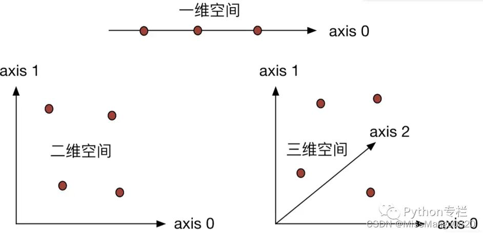
迭代顺序：order

先以下面的数组为例，对如何实现按顺序迭代访问进行说明：

l1 = [24, 10, 12, 43, 14, 37, 43, 47, 17, 3, 42, 88, 73, 64, 21, 67, 21, 64, 22, 95, 4, 74, 4, 100]
np1 = np.array(l1).reshape(3, 2, 4)
# [[[ 24  10  12  43]
#   [ 14  37  43  47]]
#
#  [[ 17   3  42  88]
#   [ 73  64  21  67]]
#
#  [[ 21  64  22  95]
#   [  4  74   4 100]]]
#
# shape, (3, 2, 4)


for x in np.nditer(np1):
    print(x, end=",")
# 24,10,12,43,14,37,43,47,17,3,42,88,73,64,21,67,21,64,22,95,4,74,4,100,

以上示例不是使用标准 C 或者 Fortran 顺序，选择的顺序是和数组内存布局一致的，这样做是为了提升访问的效率，默认是行序优先（row-major order，或者说是 C-order）。

默认情况下只需访问每个元素，而无需考虑其特定顺序。我们可以通过迭代上述数组的转置来看到这一点，并与以 C 顺序访问数组转置的 copy 方式做对比，如下：

print(np1.T)
# [[[ 24  17  21]
#   [ 14  73   4]]
#
#  [[ 10   3  64]
#   [ 37  64  74]]
#
#  [[ 12  42  22]
#   [ 43  21   4]]
#
#  [[ 43  88  95]
#   [ 47  67 100]]]
#
# shape, (4, 2, 3)


for x in np.nditer(np1.T):
    print(x, end=",")
# 24,10,12,43,14,37,43,47,17,3,42,88,73,64,21,67,21,64,22,95,4,74,4,100,)


print(np1.T.copy(order='C'))
# [[[ 24  17  21]
#   [ 14  73   4]]
#
#  [[ 10   3  64]
#   [ 37  64  74]]
#
#  [[ 12  42  22]
#   [ 43  21   4]]
#
#  [[ 43  88  95]
#   [ 47  67 100]]]
#
# shape, (4, 2, 3)


for x in np.nditer(np1.T.copy(order='C')):
    print(x, end=",")
# 24,17,21,14,73,4,10,3,64,37,64,74,12,42,22,43,21,4,43,88,95,47,67,100,

从上述例子可以看出，np1 和 np1.T 的遍历顺序是一样的，也就是他们在内存中的存储顺序也是一样的。

但是 numpy.copy 做了特殊处理，它拷贝的时候不是直接把对方的内存复制，而是按照上面 order 指定的顺序逐一拷贝。np1.T.copy(order = 'C') 的遍历结果是不同的，那是因为它和前两种的存储方式是不一样的，默认是按行访问。

行

用法

np.nditer(a.T, order='C')

示例

np1 = np.array(l1).reshape(3, 2, 4)
# print(np1)
# [[[ 24  10  12  43]
#   [ 14  37  43  47]]
#
#  [[ 17   3  42  88]
#   [ 73  64  21  67]]
#
#  [[ 21  64  22  95]
#   [  4  74   4 100]]]
#
# shape, (3, 2, 4)


np1T = np1.T
# [[[ 24  17  21]
#   [ 14  73   4]]
#
#  [[ 10   3  64]
#   [ 37  64  74]]
#
#  [[ 12  42  22]
#   [ 43  21   4]]
#
#  [[ 43  88  95]
#   [ 47  67 100]]]
#
# shape, (4, 2, 3)


np1TcopyC = np1.T.copy(order='C')
# [[[ 24  17  21]
#   [ 14  73   4]]
#
#  [[ 10   3  64]
#   [ 37  64  74]]
#
#  [[ 12  42  22]
#   [ 43  21   4]]
#
#  [[ 43  88  95]
#   [ 47  67 100]]]
#
# shape, (4, 2, 3)


for x in np.nditer(np1TcopyC):
    print(x, end="," )
    # x.shape, ()
    # x type, <class 'numpy.ndarray'>
# 24,17,21,14,73,4,10,3,64,37,64,74,12,42,22,43,21,4,43,88,95,47,67,100,

列

用法

np.nditer(a, order='F')

示例

np1 = np.array(l1).reshape(3, 2, 4)
# print(np1)
# [[[ 24  10  12  43]
#   [ 14  37  43  47]]
#
#  [[ 17   3  42  88]
#   [ 73  64  21  67]]
#
#  [[ 21  64  22  95]
#   [  4  74   4 100]]]
#
# shape, (3, 2, 4)


np1T = np1.T
# [[[ 24  17  21]
#   [ 14  73   4]]
#
#  [[ 10   3  64]
#   [ 37  64  74]]
#
#  [[ 12  42  22]
#   [ 43  21   4]]
#
#  [[ 43  88  95]
#   [ 47  67 100]]]
#
# shape, (4, 2, 3)


np1TcopyF = np1.T.copy(order='F')
# [[[ 24  17  21]
#   [ 14  73   4]]
#
#  [[ 10   3  64]
#   [ 37  64  74]]
#
#  [[ 12  42  22]
#   [ 43  21   4]]
#
#  [[ 43  88  95]
#   [ 47  67 100]]]
#
# shape, (4, 2, 3)


for x in np.nditer(np1TcopyF):
    print(x, end="," )
    # x.shape, ()
    # x type, <class 'numpy.ndarray'>
# 24,10,12,43,14,37,43,47,17,3,42,88,73,64,21,67,21,64,22,95,4,74,4,100,

示例

np2 = np.arange(0, 60, 5).reshape(3, 4)
# [[ 0  5 10 15]
#  [20 25 30 35]
#  [40 45 50 55]]
#
# shape, (3, 4)


for x in np.nditer(np2, order='C'):
    print(x, end=",")
# 0,5,10,15,20,25,30,35,40,45,50,55,


for x in np.nditer(np2, order='F'):
    print(x, end=",")
# 0,20,40,5,25,45,10,30,50,15,35,55,

迭代维度：flags

多维

访问

用法

1. 基本迭代参数 flags=['mulit_index']，可输出自身坐标 it.multi_index。multi_index 表示对 x 进行多重索引。
   print("%d <%s>" % (it[0], it.multi_index)) 表示输出元素的索引，可以看到输出的结果都是 index。
   it.iternext() 表示进入下一次迭代，如果不加这一句的话，输出的结果就一直是不间断地输出同一个结果。

2. 基本迭代参数 flags=['external_loop] 可以指定顺序对数组进行访问。numpy 实例本身的存储顺序不会因为转置或 order = 'C' 或 'F' 而改变。只是 numpy 实例中，存储了一个默认的访问顺序的字段。
   可以在循环中另外指定顺序，如果未指定，则按照数组的内置 order 顺序访问。
   当数组的 order 与在循环中指定的 order 顺序不同时，打印为多个一维数组，当相同时，是整个一个一维数组。

示例

multi_index

np2 = np.arange(0, 60, 5).reshape(3, 4)
# [[ 0  5 10 15]
#  [20 25 30 35]
#  [40 45 50 55]]
#
# shape, (3, 4)


it = np.nditer(np2, flags=['multi_index'], op_flags=['readwrite'])
while not it.finished:
	print("%d <%s>" % (it[0], it.multi_index))
	# `it` type, <class 'numpy.nditer'>
    # `it` shape, (3, 4)
	it.iternext()
# 0 <(0, 0)>
# 5 <(0, 1)>
# 10 <(0, 2)>
# 15 <(0, 3)>
# 20 <(1, 0)>
# 25 <(1, 1)>
# 30 <(1, 2)>
# 35 <(1, 3)>
# 40 <(2, 0)>
# 45 <(2, 1)>
# 50 <(2, 2)>
# 55 <(2, 3)>

external_loop

np2 = np.arange(0, 60, 5).reshape(3, 4)
# [[ 0  5 10 15]
#  [20 25 30 35]
#  [40 45 50 55]]
#
# shape, (3, 4)


for x in np.nditer(np2, flags=['external_loop'], order='F'):
    print(x, end=',')
    # shape, (3,)
    # type, <class 'numpy.ndarray'>
# [ 0 20 40],[ 5 25 45],[10 30 50],[15 35 55],


for x in np.nditer(np2, flags=['external_loop'], order='C'):
    print(x, end=',')
    # shape, (12,)
    # type, <class 'numpy.ndarray'>
# [ 0  5 10 15 20 25 30 35 40 45 50 55],

单维

访问

用法

基本迭代参数 flags=['f_index'] 或者 flags=['c_index']，可输出自身坐标 it.index。
f_index 和 c_index 表示对 x 进行单维索引。

示例

f_index

np2 = np.arange(0, 60, 5).reshape(3, 4)
# [[ 0  5 10 15]
#  [20 25 30 35]
#  [40 45 50 55]]
#
# shape, (3, 4)


it = np.nditer(np2, flags=['f_index'])
while not it.finished:
	print("%d <%s>" % (it[0], it.index))
    # `it` type, <class 'numpy.nditer'>
    # `it` shape, (4, 3)
	it.iternext()
# 0 <0>
# 5 <3>
# 10 <6>
# 15 <9>
# 20 <1>
# 25 <4>
# 30 <7>
# 35 <10>
# 40 <2>
# 45 <5>
# 50 <8>
# 55 <11>


for x in np.nditer(np2, order='F'):
    print(x, end=',')
    # `` type, <class 'numpy.ndarray'>
    # `` shape, ()
# 0,20,40,5,25,45,10,30,50,15,35,55,

比如，np2 数组中的元素 25 通过迭代器可以得到其索引为 4，再通过 F 迭代顺序可确认 25 的索引确实为 4。

c_index

np2 = np.arange(0, 60, 5).reshape(3, 4)
# [[ 0  5 10 15]
#  [20 25 30 35]
#  [40 45 50 55]]
#
# shape, (3, 4)


it = np.nditer(np2, flags=['c_index'])
while not it.finished:
	print("%d <%s>" % (it[0], it.index))
    # `it` type, <class 'numpy.nditer'>
    # `it` shape, (12,)
	it.iternext()
# 0 <0>
# 5 <1>
# 10 <2>
# 15 <3>
# 20 <4>
# 25 <5>
# 30 <6>
# 35 <7>
# 40 <8>
# 45 <9>
# 50 <10>
# 55 <11>


for x in np.nditer(np2, order='C'):
    print(x, end=',')
    # `` type, <class 'numpy.ndarray'>
    # `` shape, ()
# 0,5,10,15,20,25,30,35,40,45,50,55,

比如，np2 数组中的元素 25 通过迭代器可以得到其索引为 5，再通过 C 迭代顺序可确认 25 的索引确实为 5。

external_loop

np2 = np.arange(0, 60, 5).reshape(3, 4)
# [[ 0  5 10 15]
#  [20 25 30 35]
#  [40 45 50 55]]
#
# shape, (3, 4)


for x in np.nditer(np2, flags=['external_loop'], order='F'):
    print(x, end=',')
    # shape, (3,)
    # type, <class 'numpy.ndarray'>
# [ 0 20 40],[ 5 25 45],[10 30 50],[15 35 55],

迭代修改：op_flags

用法

nditer 对象有另一个可选参数 op_flags。

默认情况下，nditer 将视待迭代遍历的数组为只读对象（read-only），为了在遍历数组的同时，实现对数组元素值得修改，必须指定 read-write 或者 read-only 的模式。op_flags=['readwrite'] 表示不仅可以对数组进行 read（读取），还可以 write（写入），即相当于在创建这个迭代器的时候，就规定好了有哪些权限 ⁵⁰。

示例

np2 = np.arange(0, 60, 5).reshape(3, 4)
# [[ 0  5 10 15]
#  [20 25 30 35]
#  [40 45 50 55]]
#
# shape, (3, 4)


for x in np.nditer(np2, op_flags=['readwrite']):
    x[...] = 2*x
# [[  0  10  20  30]
#  [ 40  50  60  70]
#  [ 80  90 100 110]]
# 
# shape, (3, 4)

广播迭代

用法

如果两个数组是可广播的，nditer 组合对象能够同时迭代它们。

假设数组 np2 的维度为 3X4，数组 np1 的维度为 1X4，则使用以下迭代器（数组 np1 被广播到 np1 的大小）。

示例

np1 = np.arange(10, 50, 10).reshape(1, 4)
# [[10 20 30 40]]
#
# shape, (1, 4)


np2 = np.arange(0, 60, 5).reshape(3, 4)
# [[ 0  5 10 15]
#  [20 25 30 35]
#  [40 45 50 55]]
#
# shape, (3, 4)


for x, y in np.nditer([np2, np1]):
    print("%d -- %d"  %  (x,y), end="\n" )
    # `x` 和 `y` shape, () ()
    # `x` 和 `y` type, <class 'numpy.ndarray'>
# 0 -- 10
# 5 -- 20
# 10 -- 30
# 15 -- 40
# 20 -- 10
# 25 -- 20
# 30 -- 30
# 35 -- 40
# 40 -- 10
# 45 -- 20
# 50 -- 30
# 55 -- 40

---

---

参考链接

NumPy官方文档
NumPy 中文文档
pandas 在某个列表中的值 筛选列_数据处理-Pandas&Numpy大法

基本操作

数据生成与复制、重复

NumPy 从数值范围创建数组

属性与统计、运算

Numpy Isnan（）函数示例| Python中的Np Isnan
python编程之np.isnan()的用法

% 导出及导入和格式转换

% 操作

多数组

比较

Numpy的比较运算

合并

如何追加一个NumPy数组到一个NumPy数组？

包含

todo

Numpy array数据的增、删、改、查实例
numpy 使用delete根据index删除array里面的数据

Python创建二维数组的正确姿势
NumPy 按数字范围创建数组
numpy选取满足特定条件的元素numpy.extract
Python numpy 提取矩阵的某一行或某一列

---

1. python︱numpy、array——高级matrix（替换、重复、格式转换、切片） ↩︎

2. Numpy数组中的运算与拼接
   python︱numpy、array——高级matrix（替换、重复、格式转换、切片）
   Python numpy ndarray.itemset用法及代碼示例
   Numpy库学习—squeeze()函数
   numpy中的ravel()、flatten()、squeeze()的用法与区别
   numpy.maximum ↩︎ ↩︎

3. Python 中列表中的每个数字中减去一个值 ↩︎

4. Python Numpy数组保存 ↩︎

5. 按行将numpy数组保存到txt文件 ↩︎

6. 如何在Python中将列表元素添加/删除/插入 ↩︎

7. NumPy数组元素的添加和删除 ↩︎ ↩︎

8. numpy矩阵添加一行或一列 ↩︎

9. PYthon 从numpy数组去除重复元素，行或列 ↩︎

10. Python numpy unique用法及代码示例 ↩︎

11. numpy中delete的使用方法 ↩︎

12. 18_NumPy数组ndarray中提取，删除满足条件的元素，行和列
    Python numpy ndarray.itemset用法及代碼示例
    numpy 进行数组的拼接，分别在行和列上合并
    numpy中的数组之间进行集合运算
    NumPy二维数组-行向量、列向量
    python 二维数组找特定行 find row in 2d numpy array
    从Numpy中的ascontiguousarray说起?
    Numpy学习笔记 （基于Numpy 1.11.0） ↩︎ ↩︎

13. Python numpy.unique函数方法的使用 ↩︎

14. Python numpy 提取矩阵的某一行或某一列 ↩︎

15. Python：NumPy-随机抽样 ↩︎

16. [Python] 随机抽样 ↩︎

17. Numpy中 np.random.shuffle()与np.random.permutation()的用法和区别 ↩︎ ↩︎

18. Python不重复批量随机抽样 random.sample() 和 numpy.random.choice() 的优缺点 ↩︎

19. np.random.uniform()的用法 ↩︎

20. Python生成随机数和numpy生成随机数 ↩︎

21. python机器学习库numpy—7.2、生成随机数-正态分布 ↩︎

22. python numpy中生成正态分布的随机数 ↩︎

23. numpy 生成满足正态分布的随机数 ↩︎

24. 机器学习必须要会的：方差、标准差、相对标准偏差、正态分布的概念 ↩︎

25. NumPy排序和搜索功能 ↩︎

26. numpy 多级排序 ：lexsort 函数详解 ↩︎

27. numpy.lexsort超详细解释 ↩︎

28. Python numpy.argpartition用法及代碼示例 ↩︎

29. numpyargpartition实例详解 ↩︎

30. numpy中的argpartition用法 ↩︎

31. python numpy 矩阵左右翻转/上下翻转 ↩︎

32. NumPy 排序、条件刷选函数 ↩︎

33. 在 Python 中找到列表中元素的索引 ↩︎

34. numpy.argwhere 与 numpy.where的区别 ↩︎

35. python 使用numpy实现从二维数组中找出行（子数组）为特定值的索引 ↩︎

36. python输出list最大值_python如何获得list或numpy数组中最大元素对应的索引 ↩︎

37. Python找出矩阵中最大值的位置 ↩︎

38. 【python】np.where和np.argwhere、np.squeeze ↩︎

39. max与argmax的区别 ↩︎

40. python - 如何计算numpy数组中元素的频率？ - 探索字符串 ↩︎

41. python如何判断两个数组完全相等？ ↩︎

42. np.isin判断数组元素在另一数组中是否存在 ↩︎

43. python-numpy.array中，any()和all()方法介绍 ↩︎ ↩︎

44. numpy.all()函数 与 numpy.any()函数 ↩︎ ↩︎

45. numpy数组的拼接(扩维拼接和非扩维拼接) ↩︎

46. numpy数组拼接方法介绍(concatenate)—一次性完成多个数组的拼接 ↩︎

47. 【冰糖Python】numpy 差集、异或集、并集、交集 setdiff1d() setxor1d() union1d() intersect1d() ↩︎

48. NumPy 迭代数组 ↩︎

49. it = np.nditer(x, flags=[‘multi_index’], op_flags=[‘readwrite’]) ↩︎

50. np.nditer、flags=[‘multi_index‘] 用法 ↩︎