


Fine-Tuning and Guidance
在这一节的笔记本中,我们将讲解两种主要的基于现有模型实现改造的方法:
- 通过微调(fine-tuning),我们将在新的数据集上重新训练已有的模型,来改变它原有的输出类型
- 通过引导(guidance),我们将在推理阶段引导现有模型的生成过程,以此来获取额外的控制
你将学到:
在阅读完这一节笔记本后,你将学会:
- 创建一个采样循环,并使用调度器(scheduler)更快地生成样本
- 在新数据集上微调一个现有的扩散模型,这包括:
- 使用累积梯度的方法去应对训练的 batch 太小所带来的一些问题
- 在训练过程中,将样本上传到 Weights and Biases 来记录日志,以此来监控训练过程(通过附加的实例脚本程序)
- 将最终结果管线(pipeline)保存下来,并上传到Hub
- 通过新加的损失函数来引导采样过程,以此对现有模型施加控制,这包括:
- 通过一个简单的基于颜色的损失来探索不同的引导方法
- 使用 CLIP,用文本来引导生成过程
- 用 Gradio 和 🤗 Spaces 来分享你的定制的采样循环
❓如果你有问题,请在 Hugging Face Discord 的 #diffusion-models-class 频道提出。如果你还没有 Hugging Face 的账号,你可以在这里注册:https://huggingface.co/join/discord
配置过程和需要引入的库
为了将你的微调过的模型保存到 Hugging Face Hub 上,你需要使用一个具有写权限的访问令牌来登录。下列代码将会引导你登陆并连接上你的账号的相关令牌页。如果在模型训练过程中,你想使用训练脚本将样本记录到日志,你也需要一个 Weights and Biases 账号 —— 同样地,这些代码也会在需要的时候引导你登录。
此外,你唯一需要配置的就是安装几个依赖,并在程序中引入我们需要的东西然后制定好我们将使用的计算设备。
!pip install -qq diffusers datasets accelerate wandb open-clip-torch
# Code to log in to the Hugging Face Hub, needed for sharing models
# Make sure you use a token with WRITE access
from huggingface_hub import notebook_login

notebook_login()
VBox(children=(HTML(value='<center> <img\nsrc=https://huggingface.co/front/assets/huggingface_logo-noborder.sv…
import numpy as np
import torch
import torch.nn.functional as F
import torchvision
from datasets import load_dataset
from diffusers import DDIMScheduler, DDPMPipeline
from matplotlib import pyplot as plt
from PIL import Image
from torchvision import transforms
from tqdm.auto import tqdm
device = (
    "mps"
    if torch.backends.mps.is_available()
    else "cuda"
    if torch.cuda.is_available()
    else "cpu"
)
载入一个预训练过的管线
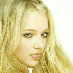
在本节笔记本的开始,我们先载入一个现有的管线,来看看我们能用它做些什么:
image_pipe = DDPMPipeline.from_pretrained("google/ddpm-celebahq-256")
image_pipe.to(device);
diffusion_pytorch_model.safetensors not found


Loading pipeline components...:   0%|          | 0/2 [00:00<?, ?it/s]
生成图像就像调用管线的__call__方法一样简单,我们像调用函数一样来试试:
images = image_pipe().images
images[0]
0%| | 0/1000 [00:00<?, ?it/s]
微调
现在玩点好玩的!给我们一个预训练过的管线(pipeline),我们怎样使用新的训练数据重训模型来生成图片?
看起来这和我们从头训练模型是几乎一样的(正如我们在第一单元所见的一样),除了我们这里是用现有模型作为初始化的。让我们实践一下看看,并额外考虑几点我们要注意的东西。
首先,数据方面,你可以尝试用 Vintage Faces 数据集 或者这些动漫人脸图片来获取和这个人脸模型的原始训练数据类似的数据。但我们现在还是先用和第一单元一样的蝴蝶数据集吧。通过以下代码来下载蝴蝶数据集,并建立一个能按批(batch)采样图片的dataloader:
# @markdown load and prepare a dataset:
# Not on Colab? Comments with #@ enable UI tweaks like headings or user inputs
# but can safely be ignored if you're working on a different platform.

dataset_name = "fashion_mnist"  # @param
dataset = load_dataset(dataset_name, split="train")
image_size = 128  # @param
batch_size = 4  # @param
preprocess = transforms.Compose(
    [
        transforms.Resize((image_size, image_size)),
        transforms.RandomHorizontalFlip(),
        transforms.ToTensor(),
        transforms.Normalize([0.5], [0.5]),
    ]
)


def transform(examples):
    images = [preprocess(image.convert("RGB")) for image in examples["image"]]
    return {"images": images}


dataset.set_transform(transform)

train_dataloader = torch.utils.data.DataLoader(
    dataset, batch_size=batch_size, shuffle=True
)

print("Previewing batch:")
batch = next(iter(train_dataloader))
grid = torchvision.utils.make_grid(batch["images"], nrow=4)
plt.imshow(grid.permute(1, 2, 0).cpu().clip(-1, 1) * 0.5 + 0.5);
Downloading builder script:   0%|          | 0.00/4.83k [00:00<?, ?B/s]


Downloading metadata:   0%|          | 0.00/3.13k [00:00<?, ?B/s]


Downloading readme:   0%|          | 0.00/8.85k [00:00<?, ?B/s]


Downloading data files:   0%|          | 0/4 [00:00<?, ?it/s]


Downloading data:   0%|          | 0.00/26.4M [00:00<?, ?B/s]


Downloading data:   0%|          | 0.00/29.5k [00:00<?, ?B/s]


Downloading data:   0%|          | 0.00/4.42M [00:00<?, ?B/s]


Downloading data:   0%|          | 0.00/5.15k [00:00<?, ?B/s]


Extracting data files:   0%|          | 0/4 [00:00<?, ?it/s]


Generating train split:   0%|          | 0/60000 [00:00<?, ? examples/s]


Generating test split:   0%|          | 0/10000 [00:00<?, ? examples/s]


Previewing batch:

考虑因素1: 我们这里使用的 batch size 很小(只有 4),因为我们的训练是基于较大的图片尺寸的(256px),并且我们的模型也很大,如果我们的 batch size 太高,GPU 的内存可能会不够用了。你可以减小图片尺寸,换取更大的 batch size 来加速训练,但这里的模型一开始都是基于生成 256px 尺寸的图片来设计和训练的。
现在我们看看训练循环。我们把要优化的目标参数设定为image_pipe.unet.parameters(),以此来更新预训练过的模型的权重。其它部分的代码基本上和第一单元例子中的对应部分一样。在 Colab 上跑的话,大约需要10分钟,你可以趁这个时间喝杯茶休息一下。
num_epochs = 2  # @param
lr = 1e-5  # 2param
grad_accumulation_steps = 2  # @param

optimizer = torch.optim.AdamW(image_pipe.unet.parameters(), lr=lr)

losses = []

for epoch in range(num_epochs):
    for step, batch in tqdm(enumerate(train_dataloader), total=len(train_dataloader)):
        clean_images = batch["images"].to(device)
        # Sample noise to add to the images
        noise = torch.randn(clean_images.shape).to(clean_images.device)
        bs = clean_images.shape[0]

        # Sample a random timestep for each image
        timesteps = torch.randint(
            0,
            image_pipe.scheduler.num_train_timesteps,
            (bs,),
            device=clean_images.device,
        ).long()

        # Add noise to the clean images according to the noise magnitude at each timestep
        # (this is the forward diffusion process)
        noisy_images = image_pipe.scheduler.add_noise(clean_images, noise, timesteps)

        # Get the model prediction for the noise
        noise_pred = image_pipe.unet(noisy_images, timesteps, return_dict=False)[0]

        # Compare the prediction with the actual noise:
        loss = F.mse_loss(
            noise_pred, noise
        )  # NB - trying to predict noise (eps) not (noisy_ims-clean_ims) or just (clean_ims)

        # Store for later plotting
        losses.append(loss.item())

        # Update the model parameters with the optimizer based on this loss
        loss.backward(loss)

        # Gradient accumulation:
        if (step + 1) % grad_accumulation_steps == 0:
            optimizer.step()
            optimizer.zero_grad()

    print(
        f"Epoch {epoch} average loss: {sum(losses[-len(train_dataloader):])/len(train_dataloader)}"
    )

# Plot the loss curve:
plt.plot(losses)
  0%|          | 0/15000 [00:00<?, ?it/s]


F:\software\Anaconda\envs\test\lib\site-packages\diffusers\configuration_utils.py:134: FutureWarning: Accessing config attribute `num_train_timesteps` directly via 'DDPMScheduler' object attribute is deprecated. Please access 'num_train_timesteps' over 'DDPMScheduler's config object instead, e.g. 'scheduler.config.num_train_timesteps'.
  deprecate("direct config name access", "1.0.0", deprecation_message, standard_warn=False)


Epoch 0 average loss: 0.002848186818284254


  0%|          | 0/15000 [00:00<?, ?it/s]


Epoch 1 average loss: 0.0022448867649994403


[<matplotlib.lines.Line2D at 0x17b2b7fde50>]
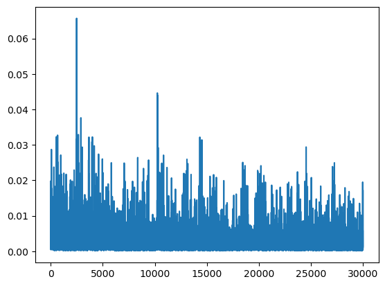
考虑因素2: 我们的损失值曲线简直像噪声一样混乱!这是因为每一次迭代我们都只用了四个训练样本,而且加到它们上面的噪声水平还都是随机挑选的。这对于训练来讲并不理想。一种弥补的措施是,我们使用一个非常小的学习率,限制每次更新的幅度。但我们还有一个更好的方法,既能得到和使用更大的 batch size 一样的收益,又不需要让我们的内存爆掉。
点击这里看看:gradient accumulation。如果我们多运行几次loss.backward()后再调用optimizer.step()和optimizer.zero_grad(),PyTorch 就会把梯度累积(加和)起来,这样多个批次的数据产生的更新信号就会被高效地融合在一起,产出一个单独的(更好的)梯度估计用于参数更新。这样做会减少参数更新的总次数,就正如我们使用更大的 batch size 时希望看到的一样。梯度累积是一个很多框架都会替你做的事情(比如这里:🤗 Accelerate makes this easy),但这里我们从头实现一遍也挺好的,因为这对你在 GPU 内存受限时训练模型非常有帮助。正如你在上面代码中看到的那样(在注释 # Gradient accumulation 后),其实也不需要你写很多代码。
# 练习:试试你能不能把梯度累积加到第一单元的训练循环中
# 怎么做呢?你应该怎么基于梯度累积的步数来调整学习率?
# 学习率应该和之前一样吗?
考虑因素3: 即使这样,我们的训练还是挺慢的,而且每遍历完一轮数据集才打印出一行更新,这也不足以让我们知道我们的训练到底怎样了。我们也许还应该:
- 训练过程中时不时地生成点图像样本,供我们检查模型性能
- 在训练过程中,把诸如损失值和生成的图片样本在内的一些东西记录到日志里。你可以使用诸如 Weights and Biases 或 tensorboard 之类的工具
我创建了一个快速的脚本程序(finetune_model.py),使用了上述的训练代码并加入了少量日志记录功能。你可以在这里看看一次训练的日志:
%wandb johnowhitaker/dm_finetune/2upaa341 # You'll need a W&B account for this to work - skip if you don't want to log in
观察随着训练进展生成的样本图片如何变化也挺好玩 —— 即使从损失值看它好像并没有改进,但我们也能看到一个从原有图像分布(卧室图片)到新的数据集(wikiart 数据集)逐渐演变的过程。在这一节笔记本最后还有一些被注释掉的用于微调的代码,可以使用该脚本程序替代你运行上面的代码块。
# 练习: 看看你能不能修改第一单元的官方示例训练脚本程序
# 尝试使用预训练的模型,而不是从头开始训练
# 对比一下上面链接的最小化脚本 —— 对比一下哪些额外功能是最小化脚本没有的?
用这个模型生成点图片,我们可以看到这些脸看起来极其奇怪!
# @markdown Generate and plot some images:
x = torch.randn(8, 3, 256, 256).to(device)  # Batch of 8
for i, t in tqdm(enumerate(scheduler.timesteps)):
    model_input = scheduler.scale_model_input(x, t)
    with torch.no_grad():
        noise_pred = image_pipe.unet(model_input, t)["sample"]
    x = scheduler.step(noise_pred, t, x).prev_sample
grid = torchvision.utils.make_grid(x, nrow=4)
plt.imshow(grid.permute(1, 2, 0).cpu().clip(-1, 1) * 0.5 + 0.5);
0it [00:00, ?it/s]
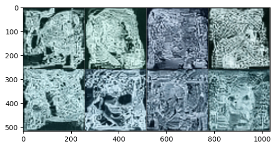
考虑因素4: 微调这个过程可能是难以预知的。如果我们训练很长时间,我们也许能看见一些生成得很完美的蝴蝶,但中间过程从模型自身讲也极其有趣,尤其是你对艺术风格感兴趣时!你可以试试短时间或长时间地观察一下训练过程,并试着该百年学习率,看看这会怎么影响模型的最终输出。
这个fine-tune跑了很久,结果果真出人意料,后面有空再尝试改变参数,后续保存到hugging face报了序列化错误,先做个笔记,再慢慢查原因。


 2835
2835


 被折叠的 条评论
为什么被折叠?
被折叠的 条评论
为什么被折叠?
 到【灌水乐园】发言


