吴恩达机器学习作业6---Support Vector Machines（上）

代码分析

1. SVM with linear Kernels

首先带入类库

import numpy as np
import matplotlib.pyplot as plt
import scipy.io #导入mat文件
import scipy.optimize #fmin_cg to train the linear regression
from sklearn import svm #SVM software

%matplotlib inline

导入数据

datafile = 'data/ex6data1.mat'
mat = scipy.io.loadmat( datafile )
#Training set
X, y = mat['X'], mat['y']
#不需要再X前插入全为1的一列了，SVM软件会自动为我们做的
#将数据集分为pos类和neg类
pos = np.array([X[i] for i in range(X.shape[0]) if y[i] == 1])
neg = np.array([X[i] for i in range(X.shape[0]) if y[i] == 0])

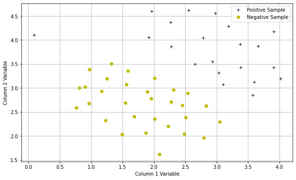
可视化数据

def plotData(pos,neg):
    plt.figure(figsize=(10,6))
    plt.plot(pos[:,0],pos[:,1],'k+',label='Positive Sample')
    plt.plot(neg[:,0],neg[:,1],'yo',label='Negative Sample')
    plt.xlabel('Column 1 Variable')
    plt.ylabel('Column 2 Variable')
    plt.legend()
    plt.grid(True)
    
plotData(pos,neg)

编写绘制决策界限的函数

#画出svm的决策界限
def plotBoundary(my_svm, xmin, xmax, ymin, ymax):
    xvals = np.linspace(xmin,xmax,100)
    yvals = np.linspace(ymin,ymax,100)
    zvals = np.zeros((len(xvals),len(yvals)))
    for i in range(len(xvals)):
        for j in range(len(yvals)):
            zvals[i][j] = float(my_svm.predict(np.array([xvals[i],yvals[j]]).reshape(1,-1)))#这里需要reshape
    zvals = zvals.transpose()
    u, v = np.meshgrid( xvals, yvals )
    #在值为0处画一条等高线
    mycontour = plt.contour( xvals, yvals, zvals,[0])
    plt.title("Decision Boundary")

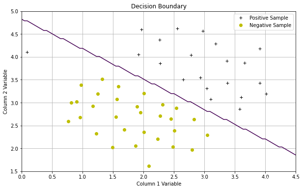
测试C=1时的SVM分类效果

#首先创建一个SVM，C=1，线性核
linear_svm = svm.SVC(C=1, kernel='linear')
#训练svm
linear_svm.fit( X, y.flatten() )
#画出决策界限
plotData(pos,neg)
plotBoundary(linear_svm,0,4.5,1.5,5)

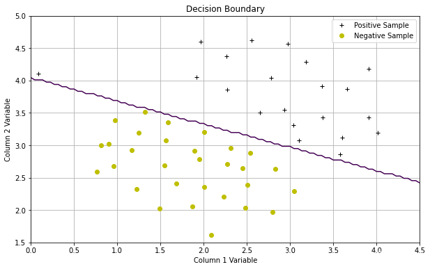
测试C=100时的SVM分类效果

#C为100时的svm
linear_svm = svm.SVC(C=100, kernel='linear')
linear_svm.fit( X, y.flatten() )
plotData(pos,neg)
plotBoundary(linear_svm,0,4.5,1.5,5)

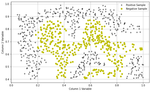
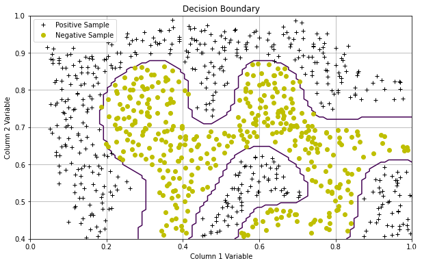
2. SVM with Gaussian Kernels

这是高斯核函数（不用自己编写）

#高斯核函数
def gaussKernel(x1, x2, sigma):
    sigmasquared = np.power(sigma,2)
    return np.exp(-(x1-x2).T.dot(x1-x2)/(2*sigmasquared))

导入数据，并可视化

datafile = 'data/ex6data2.mat'
mat = scipy.io.loadmat( datafile )
#Training set
X, y = mat['X'], mat['y']

pos = np.array([X[i] for i in range(X.shape[0]) if y[i] == 1])
neg = np.array([X[i] for i in range(X.shape[0]) if y[i] == 0])

plotData(pos,neg)

测试

# 用高斯核函数训练svm
#rbf参数
sigma = 0.1
gamma = np.power(sigma,-2.)
gaus_svm = svm.SVC(C=1, kernel='rbf', gamma=gamma)
gaus_svm.fit( X, y.flatten() )
plotData(pos,neg)
plotBoundary(gaus_svm,0,1,.4,1.0)

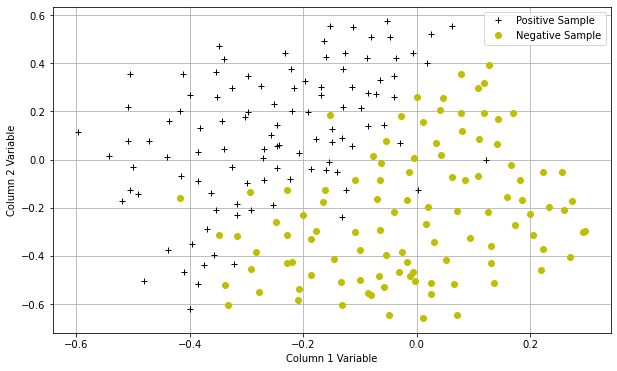
3. 高斯核SVM自动选择参数C和σ

导入数据并可视化

datafile = 'data/ex6data3.mat'
mat = scipy.io.loadmat( datafile )
#Training set
X, y = mat['X'], mat['y']
Xval, yval = mat['Xval'], mat['yval']

pos = np.array([X[i] for i in range(X.shape[0]) if y[i] == 1])
neg = np.array([X[i] for i in range(X.shape[0]) if y[i] == 0])

plotData(pos,neg)

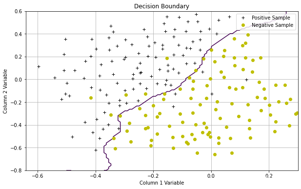
通过build-in 的评分函数自动选择最优的参数

#选择最好的C和σ
Cvalues = (0.01, 0.03, 0.1, 0.3, 1., 3., 10., 30.)
sigmavalues = Cvalues
best_pair, best_score = (0, 0), 0

for Cvalue in Cvalues:
    for sigmavalue in sigmavalues:
        #训练SVM
        gamma = np.power(sigmavalue,-2.)
        gaus_svm = svm.SVC(C=Cvalue, kernel='rbf', gamma=gamma)
        gaus_svm.fit( X, y.flatten() )
        #这是svm内置的评分工具，评价C和σ
        this_score = gaus_svm.score(Xval,yval)
        #print(this_score)
        if this_score > best_score:
            best_score = this_score
            best_pair = (Cvalue, sigmavalue)
            
print ("Best C, sigma pair is (%f, %f) with a score of %f."%(best_pair[0],best_pair[1],best_score))

输出：Best C, sigma pair is (0.300000, 0.100000) with a score of 0.965000.

测试

gaus_svm = svm.SVC(C=best_pair[0], kernel='rbf', gamma = np.power(best_pair[1],-2.))
gaus_svm.fit( X, y.flatten() )
plotData(pos,neg)
plotBoundary(gaus_svm,-.5,.3,-0.8,.6)

数据集

ex6data1.mat
ex6data2.mat
ex6data3.mat
可以上kaggle上查，这里偷个懒