非监督学习+NLTK实现基于摘要的论文分类

所需要的技术：
聚类分析-Hierarchical Clustering
自然语言处理中的tokenization ，stemming，TFIDF
数据集链接论文分类数据集
(5.16日，刚上传数据，可能还看不到）

首先说一下Tfidf
其中TF是词频（Term Frequency）的意思，指的是某一个词语在给定文件中的频率

IDF指的是逆向文件频率（Inverse Document Frequency）是一个词语普遍重要性的度量。某一特定词语的idf，可以由总文件数目除以包含该词语之文件的数目，再将得到的商取以10为底的对数得到。

举个例子。假如一篇文件的总词语数是100个，而词语“母牛”出现了3次，那么“母牛”一词在该文件中的词频就是3/100=0.03。而IDF的是以文件集的文件总数，除以出现“母牛”一词的文件数。所以，如果“母牛”一词在1,000份文件出现过，而文件总数是10,000,000份的话，其逆向文件频率就是lg（10,000,000 / 1,000）=4。最后的tf-idf的分数为0.03 * 4=0.12

首先从代码角度理解一下tfidf
先来两个数据意思一下

corpus=[
    'I love you so much',
    ' Like a paradise missing',
    'Good enough to stop',
    'Too bad or too good, it doesnt matter'
]

from sklearn.feature_extraction.text import TfidfVectorizer
xtf=TfidfVectorizer()
X_co =xtf.fit_transform(corpus)
print(xtf.get_feature_names())
print(X_co)
print(xtf.vocabulary_)

这里corpus里面一共4句话，所以样本数量为4.
先看一下输出结果：

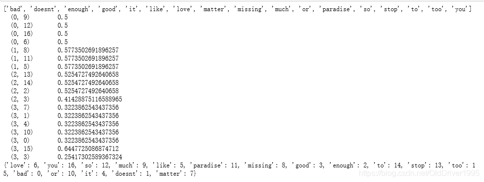
如果这里查看x_co.shape 你就会发现它的维度正好是样本数4 * feature_names的数量，而这一长串的输出结果好像并不符合这个维度。实际上它是这样表示的，（0，9）表示第0个句子（I love you so much)中9号词语（much）的tfidf为0.5。而后面的（0，12），（0，16），（0，6)正好对应（you so much)这三个词。。注意没有 I 这个词。

把他转成DataFrame看就能够理解了：

table = pd.DataFrame(X_co.toarray(), columns=xtf.get_feature_names())
table.T

图像如下：
可以看到每个词对应的句子，以及他的tfidf

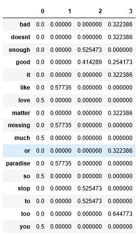
由于print的时候，0直接不显示，这就解释了为什么他看起来跟x_co的shape不太吻合

然后来看第一句话四个词语的tfidf，由于他们在这句话中各出现一次，并且在所有文本中也只存在于这句话，所以他们的tfidf也相等。

文本分类的代码实现：
这个data 一共有五列，分别是paper_id, paper_title, paper_keywords, abstract和session。
这里需要用来做分析的是abstract这一列，因为它包含的信息最多，其他几列较少，不适合分类。

import numpy as np
import pandas as pd
Data=pd.read_csv("./文件地址")
abstract=Data['abstract']
titles=Data['paper_title']

然后是定义tokenize和stem，直接使用nltk包

import nltk
from nltk.stem.snowball import SnowballStemmer
import re
stemmer = SnowballStemmer("english")
nltk.download('punkt')
def tokenize_and_stem(text):
    
    tokens = [word for sent in nltk.sent_tokenize(text) for word in nltk.word_tokenize(sent)]
    filtered_tokens = []
    
    for token in tokens:
        if re.search('[a-zA-Z]', token):
            filtered_tokens.append(token)
    stems = [stemmer.stem(t) for t in filtered_tokens]
    return stems

接着实现tfidf向量化

from sklearn.feature_extraction.text import TfidfVectorizer
from sklearn.metrics.pairwise import cosine_similarity

tfidf_vectorizer = TfidfVectorizer(max_df=0.8, max_features=200000,
min_df=0.2, stop_words='english',use_idf=True,
 tokenizer=tokenize_and_stem, ngram_range=(1,3))
 
tfidf_matrix = tfidf_vectorizer.fit_transform(abstract)
dist = 1 - cosine_similarity(tfidf_matrix) #shape 105*105

from scipy.cluster.hierarchy import complete, dendrogram ,linkage
linkage_matrix = complete(dist) #define the linkage_matrix using ward clustering pre-computed distances #dim=105 * 4
fig, ax = plt.subplots(figsize=(12, 40)) # set size
ax = dendrogram(linkage_matrix, orientation="left", labels=np.array(titles))
#到这里就已经完成了
#下面是设定输出的style
plt.tick_params(\
    axis= 'x',          # changes apply to the x-axis
    which='both',      # both major and minor ticks are affected
    bottom='off',      # ticks along the bottom edge are off
    top='off',         # ticks along the top edge are off
    labelbottom='off',
    labelsize=15
    )
plt.tick_params(\
    axis= 'y',          # changes apply to the y-axis
    labelsize=15
    )
plt.tight_layout() #show plot with tight layout

最后实现了是这个效果，实现了基于摘要提取关键字的聚类分析。

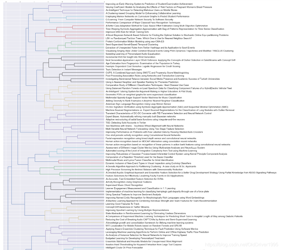
图片太长，这里只能显示一部分，如果想要保存图片，可以使用plt.savefig