深度学习复盘与论文复现C

4、Distributed training

4.1 GPU architecture

5、Recurrent neural network

RNN（Recurrent Neural Network，循环神经网络）是一种具有“记忆”功能的神经网络，它特别适合处理序列数据，如文本、语音、时间序列等。RNN通过在其内部结构中引入循环，使得网络能够捕捉序列中的时间依赖性和动态性。

5.1 The basic structure of RNN

• RNN 的核心部分是一个循环单元，它接收当前的输入 x_t 和前一个时间步的隐藏状态 h_{t-1}，然后输出一个当前时间步的隐藏状态 h_t 和一个可选的输出 y_t。隐藏状态 h_t 包含了到目前为止观察到的序列的信息，它可以被看作是网络的“记忆”。

RNN 的公式表示

在 RNN 中，隐藏状态 h_t 和输出 y_t 的计算通常使用以下公式：

• 隐藏状态的计算：h_t = f(W_xh * x_t + W_hh * h_{t-1} + b_h)
• 输出的计算（如果需要）：y_t = g(W_hy * h_t + b_y)

其中：

• f 和 g 是激活函数，如 sigmoid、tanh 或 ReLU。
• W_xh、W_hh 和 W_hy 是权重矩阵。
• b_h 和 b_y 是偏置项。

RNN 的问题

尽管 RNN 在处理序列数据方面非常有效，但它也面临一些问题：

1. 梯度消失/梯度爆炸：当处理长序列时，RNN 可能会遇到梯度消失或梯度爆炸的问题，这会导致网络难以学习长期依赖关系。
2. 计算效率：RNN 在处理每个时间步时都需要重新计算隐藏状态，这导致计算效率较低。

RNN 的变体

为了解决这些问题，研究人员提出了 RNN 的多种变体，其中最著名的是 LSTM（Long Short-Term Memory，长短期记忆）和 GRU（Gated Recurrent Unit，门控循环单元）。这些变体通过引入门控机制和内部状态来改进 RNN 的性能。

• LSTM：LSTM 通过引入输入门、遗忘门和输出门来控制信息的流动，并使用内部状态来存储长期信息。这使得 LSTM 能够更好地学习长期依赖关系。

• GRU：GRU 是 LSTM 的一个简化版本，它只包含重置门和更新门，但仍然能够捕获长期依赖关系。GRU 的计算效率通常比 LSTM 更高。

  应用场景

RNN 及其变体在许多领域都有广泛的应用，包括：

• 自然语言处理：如文本生成、机器翻译、情感分析等。
• 语音识别：将语音转换为文本。
• 时间序列预测：如股票价格预测、天气预测等。
• 音乐生成：基于旋律和节奏生成新的音乐。
• 推荐系统：根据用户的历史行为预测其未来的兴趣。

5.2 Neural networks without hidden states

• 考虑一个含单隐藏层的多层感知机。给定样本数为$n$、输入个数（特征数或特征向量维度）为$d$的小批量数据样本$\mathbf{X}\in {\mathbb{R}}^{n\times d}$。设隐藏层的激活函数为$\varphi$，那么隐藏层的输出$\mathbf{H}\in {\mathbb{R}}^{n\times h}$计算为

$$\mathbf{H}=\varphi (\mathbf{X}{\mathbf{W}}_{xh}+{\mathbf{b}}_h),$$

其中隐藏层权重参数${\mathbf{W}}_{xh}\in {\mathbb{R}}^{d\times h}$，隐藏层偏差参数 ${\mathbf{b}}_h\in {\mathbb{R}}^{1\times h}$，$h$为隐藏单元个数。上式相加的两项形状不同，因此将按照广播机制相加。把隐藏变量$\mathbf{H}$作为输出层的输入，且设输出个数为$q$（如分类问题中的类别数），输出层的输出为

$$\mathbf{O}=\mathbf{H}{\mathbf{W}}_{hq}+{\mathbf{b}}_q,$$

其中输出变量$\mathbf{O}\in {\mathbb{R}}^{n\times q}$, 输出层权重参数${\mathbf{W}}_{hq}\in {\mathbb{R}}^{h\times q}$, 输出层偏差参数${\mathbf{b}}_q\in {\mathbb{R}}^{1\times q}$。如果是分类问题，我们可以使用$\text{softmax}(\mathbf{O})$来计算输出类别的概率分布。

5.3 Recurrent neural networks with hidden states

import torch

X, W_xh = torch.randn(3, 1), torch.randn(1, 4)
H, W_hh = torch.randn(3, 4), torch.randn(4, 4)
torch.matmul(X, W_xh) + torch.matmul(H, W_hh)

输出：

tensor([[ 5.2633, -3.2288,  0.6037, -1.3321],
        [ 9.4012, -6.7830,  1.0630, -0.1809],
        [ 7.0355, -2.2361,  0.7469, -3.4667]])

• 将矩阵X和H按列（维度1）连结，连结后的矩阵形状为(3, 5)。可见，连结后矩阵在维度1的长度为矩阵X和H在维度1的长度之和（$1+4$）。然后，将矩阵W_xh和W_hh按行（维度0）连结，连结后的矩阵形状为(5, 4)。最后将两个连结后的矩阵相乘，得到与上面代码输出相同的形状为(3, 4)的矩阵。

torch.matmul(torch.cat((X, H), dim=1), torch.cat((W_xh, W_hh), dim=0))

输出：

tensor([[ 5.2633, -3.2288,  0.6037, -1.3321],
        [ 9.4012, -6.7830,  1.0630, -0.1809],
        [ 7.0355, -2.2361,  0.7469, -3.4667]])

5.4 summary

• 使用循环计算的网络即循环神经网络。
• 循环神经网络的隐藏状态可以捕捉截至当前时间步的序列的历史信息。
• 循环神经网络模型参数的数量不随时间步的增加而增长。
• 可以基于字符级循环神经网络来创建语言模型。

---

6、Language Model Dataset (lyrics from Jay Chou’s album)

• 预处理一个语言模型数据集，并将其转换成字符级循环神经网络所需要的输入格式。

6.1 Read Dataset

import torch
import random
import zipfile

with zipfile.ZipFile('../../data/jaychou_lyrics.txt.zip') as zin:
    with zin.open('jaychou_lyrics.txt') as f:
        corpus_chars = f.read().decode('utf-8')
corpus_chars[:40]

输出：

'想要有直升机\n想要和你飞到宇宙去\n想要和你融化在一起\n融化在宇宙里\n我每天每天每'

• 为了打印方便，我们把换行符替换成空格，然后仅使用前1万个字符来训练模型。

corpus_chars = corpus_chars.replace('\n', ' ').replace('\r', ' ')
corpus_chars = corpus_chars[0:10000]

6.2 Establish character index

• 我们将每个字符映射成一个从0开始的连续整数，又称索引，来方便之后的数据处理。为了得到索引，我们将数据集里所有不同字符取出来，然后将其逐一映射到索引来构造词典。接着，打印vocab_size，即词典中不同字符的个数，又称词典大小。

idx_to_char = list(set(corpus_chars))
char_to_idx = dict([(char, i) for i, char in enumerate(idx_to_char)])
vocab_size = len(char_to_idx)
vocab_size # 1027

之后，将训练数据集中每个字符转化为索引，并打印前20个字符及其对应的索引。

corpus_indices = [char_to_idx[char] for char in corpus_chars]
sample = corpus_indices[:20]
print('chars:', ''.join([idx_to_char[idx] for idx in sample]))
print('indices:', sample)

输出：

chars: 想要有直升机 想要和你飞到宇宙去 想要和
indices: [250, 164, 576, 421, 674, 653, 357, 250, 164, 850, 217, 910, 1012, 261, 275, 366, 357, 250, 164, 850]

6.3 Sampling of temporal data

• 在训练中我们需要每次随机读取小批量样本和标签。与之前章节的实验数据不同的是，时序数据的一个样本通常包含连续的字符。假设时间步数为5，样本序列为5个字符，即“想”“要”“有”“直”“升”。该样本的标签序列为这些字符分别在训练集中的下一个字符，即“要”“有”“直”“升”“机”。我们有两种方式对时序数据进行采样，分别是随机采样和相邻采样。

6.3.1 Randomize Samples

1. 参数:

   • corpus_indices: 文本序列的索引表示。通常，每个字符都被映射到一个唯一的索引。
   • batch_size: 每个批次中样本的数量。
   • num_steps: 每个样本中字符的数量（即序列长度）。
   • device: 用于存储张量的设备（如 CPU 或 GPU）。默认为 None，函数内部会根据是否有可用的 GPU 来自动选择。

2. 计算样本数量:

   • num_examples = (len(corpus_indices) - 1) // num_steps: 由于每个样本都需要num_steps个字符，且最后一个字符后面没有下一个字符，所以可用的样本数量是总字符数减去1后除以num_steps的整数部分。

3. 计算轮次大小:

   • epoch_size = num_examples // batch_size: 一个轮次（epoch）中可以包含的批次数量。

4. 打乱样本索引:

   • 使用random.shuffle(example_indices)来打乱样本索引，这样每次迭代时都可以从随机位置抽取样本。

5. 定义内部函数 _data:

   • 这个函数用于从打乱后的索引中抽取长度为num_steps的序列。

6. 选择设备:

   • 如果device为None，则根据是否有可用的 GPU 自动选择设备。

7. 迭代生成批次:

   • 对于每个批次，从打乱后的索引中抽取batch_size个样本的索引，并使用_data函数从corpus_indices中提取相应的序列。
   • X 是输入序列，其中每个序列都是长度为num_steps的字符索引列表。
   • Y 是目标序列，其中每个序列是X中对应序列的下一个字符的索引列表。
   • 使用torch.tensor将这些索引列表转换为张量，并指定数据类型为torch.float32和所选的设备。
   • 使用yield关键字将张量对（X, Y）作为生成器的一部分返回。

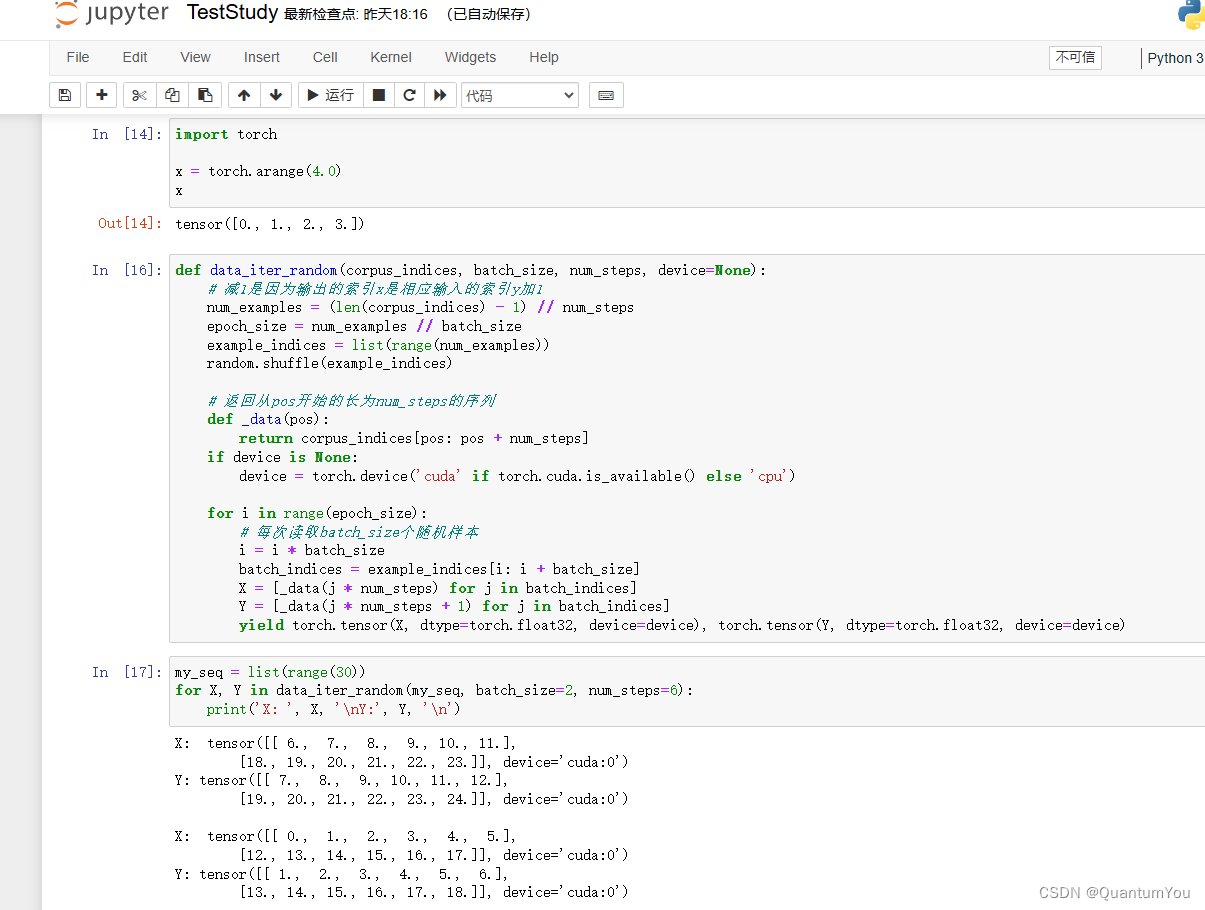
def data_iter_random(corpus_indices, batch_size, num_steps, device=None):
    # 减1是因为输出的索引x是相应输入的索引y加1
    num_examples = (len(corpus_indices) - 1) // num_steps
    epoch_size = num_examples // batch_size
    example_indices = list(range(num_examples))
    random.shuffle(example_indices)

    # 返回从pos开始的长为num_steps的序列
    def _data(pos):
        return corpus_indices[pos: pos + num_steps]
    if device is None:
        device = torch.device('cuda' if torch.cuda.is_available() else 'cpu')
    
    for i in range(epoch_size):
        # 每次读取batch_size个随机样本
        i = i * batch_size
        batch_indices = example_indices[i: i + batch_size]
        X = [_data(j * num_steps) for j in batch_indices]
        Y = [_data(j * num_steps + 1) for j in batch_indices]
        yield torch.tensor(X, dtype=torch.float32, device=device), torch.tensor(Y, dtype=torch.float32, device=device)

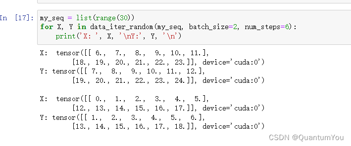
my_seq = list(range(30))
for X, Y in data_iter_random(my_seq, batch_size=2, num_steps=6):
    print('X: ', X, '\nY:', Y, '\n')

输出：

6.3.2 Adjacent sampling

• corpus_indices: 文本序列的索引表示。
• batch_size: 每个批次中样本的数量。
• num_steps: 每个样本中字符的数量（即序列长度）。
• device: 用于存储张量的设备（如 CPU 或 GPU）。默认为 None，函数内部会根据是否有可用的 GPU 来自动选择。

1. 选择设备:
   如果 device 为 None，则根据是否有可用的 GPU 自动选择设备。

2. 转换数据类型和设备:
   将 corpus_indices 转换为 PyTorch 张量，并指定数据类型为 torch.float32 和所选的设备。

3. 确定批次长度:
   由于我们想要从整个 corpus_indices 中创建连续的批次，我们首先确保 corpus_indices 的长度是 batch_size 的整数倍。如果不是，我们只取前 batch_size * batch_len 个索引，其中 batch_len 是 corpus_indices 的长度除以 batch_size 的整数部分。

4. 重新塑造数据:
   将索引张量重新塑造为二维的 (batch_size, batch_len) 形状，其中 batch_len 是每个批次中的时间步数（不是 num_steps）。

5. 确定轮次大小:
   因为每个批次中的序列是连续的，并且我们希望每个样本的长度为 num_steps，所以我们从每个批次中可以得到的最大样本数是 (batch_len - 1) // num_steps。

6. 迭代生成批次:
   对于每个轮次（epoch）中的每个步骤，我们从重新塑造的二维张量 indices 中选择连续的 num_steps 长的序列作为输入 X，并将这些序列向右移动一个位置来得到目标 Y（即每个输入序列的下一个字符）。

7. 返回数据:
   使用 yield 关键字将张量对 (X, Y) 作为生成器的一部分返回。

def data_iter_consecutive(corpus_indices, batch_size, num_steps, device=None):
    if device is None:
        device = torch.device('cuda' if torch.cuda.is_available() else 'cpu')
    corpus_indices = torch.tensor(corpus_indices, dtype=torch.float32, device=device)
    data_len = len(corpus_indices)
    batch_len = data_len // batch_size
    indices = corpus_indices[0: batch_size*batch_len].view(batch_size, batch_len)
    epoch_size = (batch_len - 1) // num_steps
    for i in range(epoch_size):
        i = i * num_steps
        X = indices[:, i: i + num_steps]
        Y = indices[:, i + 1: i + num_steps + 1]
        yield X, Y

同样的设置下，打印相邻采样每次读取的小批量样本的输入X和标签Y。相邻的两个随机小批量在原始序列上的位置相毗邻。

for X, Y in data_iter_consecutive(my_seq, batch_size=2, num_steps=6):
    print('X: ', X, '\nY:', Y, '\n')

输出：

X:  tensor([[ 0.,  1.,  2.,  3.,  4.,  5.],
        [15., 16., 17., 18., 19., 20.]]) 
Y: tensor([[ 1.,  2.,  3.,  4.,  5.,  6.],
        [16., 17., 18., 19., 20., 21.]]) 

X:  tensor([[ 6.,  7.,  8.,  9., 10., 11.],
        [21., 22., 23., 24., 25., 26.]]) 
Y: tensor([[ 7.,  8.,  9., 10., 11., 12.],
        [22., 23., 24., 25., 26., 27.]]) 

• 时序数据采样方式包括随机采样和相邻采样。使用这两种方式的循环神经网络训练在实现上略有不同。

7、Implementation of Recurrent Neural Networks from scratch

import time
import math
import numpy as np
import torch
from torch import nn, optim 
import torch.nn.functional as F

import sys
sys.path.append("..") 
import d2lzh_pytorch as d2l
device = torch.device('cuda' if torch.cuda.is_available() else 'cpu')

(corpus_indices, char_to_idx, idx_to_char, vocab_size) = d2l.load_data_jay_lyrics()

7.1 one-hot vector

• 为了将词表示成向量输入到神经网络，一个简单的办法是使用one-hot向量。假设词典中不同字符的数量为$N$（即词典大小vocab_size），每个字符已经同一个从0到$N-1$的连续整数值索引一一对应。如果一个字符的索引是整数$i$, 那么我们创建一个全0的长为$N$的向量，并将其位置为$i$的元素设成1。该向量就是对原字符的one-hot向量。下面分别展示了索引为0和2的one-hot向量，向量长度等于词典大小。

def one_hot(x, n_class, dtype=torch.float32): 
    # X shape: (batch), output shape: (batch, n_class)
    x = x.long()
    res = torch.zeros(x.shape[0], n_class, dtype=dtype, device=x.device)
    res.scatter_(1, x.view(-1, 1), 1)
    return res
    
x = torch.tensor([0, 2])
one_hot(x, vocab_size)

• 每次采样的小批量的形状是(批量大小, 时间步数)。下面的函数将这样的小批量变换成数个可以输入进网络的形状为(批量大小, 词典大小)的矩阵，矩阵个数等于时间步数。也就是说，时间步$t$的输入为${\mathbf{X}}_t\in {\mathbb{R}}^{n\times d}$，其中$n$为批量大小，$d$为输入个数，即one-hot向量长度（词典大小）。

def to_onehot(X, n_class):  
    # X shape: (batch, seq_len), output: seq_len elements of (batch, n_class)
    return [one_hot(X[:, i], n_class) for i in range(X.shape[1])]

X = torch.arange(10).view(2, 5)
inputs = to_onehot(X, vocab_size)
print(len(inputs), inputs[0].shape)

输出：

5 torch.Size([2, 1027])

7.2 Initialize model parameters

1. 参数定义：

   • num_inputs：输入层的大小，等于词汇表大小（vocab_size）。
   • num_hiddens：隐藏层的大小，这里设置为 256。
   • num_outputs：输出层的大小，也等于词汇表大小（vocab_size），因为对于每个时间步，我们都要预测一个词（通常是使用 one-hot 编码或者词嵌入）。
   • device：用于指定参数应该存储在哪个设备上（CPU 或 GPU）。

2. 打印设备：

   • 通过 print('will use', device) 打印将要使用的设备。

3. get_params 函数：

   • 该函数返回一个包含 RNN 所有参数的 nn.ParameterList。
   • 隐藏层参数：
     • W_xh：从输入层到隐藏层的权重矩阵，大小为 (num_inputs, num_hiddens)。
     • W_hh：从上一时间步的隐藏状态到当前时间步的隐藏状态的权重矩阵，大小为 (num_hiddens, num_hiddens)。
     • b_h：隐藏层的偏置向量，大小为 (num_hiddens,)。
   • 输出层参数：
     • W_hq：从隐藏层到输出层的权重矩阵，大小为 (num_hiddens, num_outputs)。
     • b_q：输出层的偏置向量，大小为 (num_outputs,)。
   • 这些参数都使用正态分布（均值为 0，标准差为 0.01）进行初始化，并使用 torch.nn.Parameter 包裹以确保它们可以作为模型的参数被优化。

num_inputs, num_hiddens, num_outputs = vocab_size, 256, vocab_size
print('will use', device)

def get_params():
    def _one(shape):
        ts = torch.tensor(np.random.normal(0, 0.01, size=shape), device=device, dtype=torch.float32)
        return torch.nn.Parameter(ts, requires_grad=True)

    # 隐藏层参数
    W_xh = _one((num_inputs, num_hiddens))
    W_hh = _one((num_hiddens, num_hiddens))
    b_h = torch.nn.Parameter(torch.zeros(num_hiddens, device=device, requires_grad=True))
    # 输出层参数
    W_hq = _one((num_hiddens, num_outputs))
    b_q = torch.nn.Parameter(torch.zeros(num_outputs, device=device, requires_grad=True))
    return nn.ParameterList([W_xh, W_hh, b_h, W_hq, b_q])

7.3 definition model

• 根据循环神经网络的计算表达式实现该模型。首先定义init_rnn_state函数来返回初始化的隐藏状态。它返回由一个形状为(批量大小, 隐藏单元个数)的值为0的NDArray组成的元组。使用元组是为了更便于处理隐藏状态含有多个NDArray的情况。

def init_rnn_state(batch_size, num_hiddens, device):
    return (torch.zeros((batch_size, num_hiddens), device=device), )

下面的rnn函数定义了在一个时间步里如何计算隐藏状态和输出。这里的激活函数使用了tanh函数。

def rnn(inputs, state, params):
    # inputs和outputs皆为num_steps个形状为(batch_size, vocab_size)的矩阵
    W_xh, W_hh, b_h, W_hq, b_q = params
    H, = state
    outputs = []
    for X in inputs:
        H = torch.tanh(torch.matmul(X, W_xh) + torch.matmul(H, W_hh) + b_h)
        Y = torch.matmul(H, W_hq) + b_q
        outputs.append(Y)
    return outputs, (H,)

state = init_rnn_state(X.shape[0], num_hiddens, device)
inputs = to_onehot(X.to(device), vocab_size)
params = get_params()
outputs, state_new = rnn(inputs, state, params)
print(len(outputs), outputs[0].shape, state_new[0].shape) 

输出：

5 torch.Size([2, 1027]) torch.Size([2, 256])

7.4 Define prediction function

1. 函数参数:

   • prefix: 一个字符串，作为预测的起始字符或字符序列。
   • num_chars: 要预测的字符数量（不包括 prefix 中的字符）。
   • rnn: RNN 模型，它应该是一个函数，接受输入、隐藏状态和参数，并返回输出和新的隐藏状态。
   • params: RNN 模型的参数。
   • init_rnn_state: 一个函数，用于初始化 RNN 的隐藏状态。
   • num_hiddens: 隐藏层的大小。
   • vocab_size: 词汇表的大小。
   • device: 设备（CPU 或 GPU），用于指定在哪里执行计算。
   • idx_to_char: 一个字典，将索引映射到字符。
   • char_to_idx: 一个字典，将字符映射到索引。

2. 初始化:

   • 使用 init_rnn_state 函数初始化 RNN 的隐藏状态。
   • 初始化一个列表 output，用于存储预测的字符索引。首先，将 prefix 的第一个字符的索引添加到 output 中。

3. 预测循环:

   • 对于 num_chars + len(prefix) - 1 次迭代（包括 prefix 中的字符和要预测的字符），执行以下操作：
     • 将上一个时间步的输出（字符索引）转换为 one-hot 编码，并作为当前时间步的输入。
     • 使用 RNN 模型、输入和当前隐藏状态计算输出和新的隐藏状态。
     • 如果当前时间步还在 prefix 之内，那么将 prefix 中的下一个字符的索引添加到 output 中。否则，从 RNN 的输出中选择概率最高的字符索引，并添加到 output 中。

4. 返回结果:

   • 使用 idx_to_char 字典将 output 中的索引转换为字符，并将这些字符连接成一个字符串返回。

def predict_rnn(prefix, num_chars, rnn, params, init_rnn_state,
                num_hiddens, vocab_size, device, idx_to_char, char_to_idx):
    state = init_rnn_state(1, num_hiddens, device)
    output = [char_to_idx[prefix[0]]]
    for t in range(num_chars + len(prefix) - 1):
        # 将上一时间步的输出作为当前时间步的输入
        X = to_onehot(torch.tensor([[output[-1]]], device=device), vocab_size)
        # 计算输出和更新隐藏状态
        (Y, state) = rnn(X, state, params)
        # 下一个时间步的输入是prefix里的字符或者当前的最佳预测字符
        if t < len(prefix) - 1:
            output.append(char_to_idx[prefix[t + 1]])
        else:
            output.append(int(Y[0].argmax(dim=1).item()))
    return ''.join([idx_to_char[i] for i in output])

• 测试一下predict_rnn函数。我们将根据前缀“分开”创作长度为10个字符（不考虑前缀长度）的一段歌词。因为模型参数为随机值，所以预测结果也是随机的。

predict_rnn('分开', 10, rnn, params, init_rnn_state, num_hiddens, vocab_size,
            device, idx_to_char, char_to_idx)

输出：

'分开西圈绪升王凝瓜必客映'

7.5 Crop gradient

• 循环神经网络中较容易出现梯度衰减或梯度爆炸。为了应对梯度爆炸，我们可以裁剪梯度（clip gradient）。假设我们把所有模型参数梯度的元素拼接成一个向量 $\mathbf{g}$，并设裁剪的阈值是$\theta$。裁剪后的梯度

$$\min \left(\frac{\theta }{\Vert \mathbf{g}\Vert },1\right)\mathbf{g}$$

的$L_2$范数不超过$\theta$。

def grad_clipping(params, theta, device):
    norm = torch.tensor([0.0], device=device)
    for param in params:
        norm += (param.grad.data ** 2).sum()
    norm = norm.sqrt().item()
    if norm > theta:
        for param in params:
            param.grad.data *= (theta / norm)

7.6 perplexity

• 通常使用困惑度（perplexity）来评价语言模型的好坏。softmax回归中交叉熵损失函数的定义。困惑度是对交叉熵损失函数做指数运算后得到的值。特别地，

• 最佳情况下，模型总是把标签类别的概率预测为1，此时困惑度为1；
• 最坏情况下，模型总是把标签类别的概率预测为0，此时困惑度为正无穷；
• 基线情况下，模型总是预测所有类别的概率都相同，此时困惑度为类别个数。

显然，任何一个有效模型的困惑度必须小于类别个数。在本例中，困惑度必须小于词典大小vocab_size。

7.7 Define model training function

1. 使用困惑度评价模型。
2. 在迭代模型参数前裁剪梯度。
3. 对时序数据采用不同采样方法将导致隐藏状态初始化的不同。

def train_and_predict_rnn(rnn, get_params, init_rnn_state, num_hiddens,
                          vocab_size, device, corpus_indices, idx_to_char,
                          char_to_idx, is_random_iter, num_epochs, num_steps,
                          lr, clipping_theta, batch_size, pred_period,
                          pred_len, prefixes):
    if is_random_iter:
        data_iter_fn = d2l.data_iter_random
    else:
        data_iter_fn = d2l.data_iter_consecutive
    params = get_params()
    loss = nn.CrossEntropyLoss()

    for epoch in range(num_epochs):
        if not is_random_iter:  # 如使用相邻采样，在epoch开始时初始化隐藏状态
            state = init_rnn_state(batch_size, num_hiddens, device)
        l_sum, n, start = 0.0, 0, time.time()
        data_iter = data_iter_fn(corpus_indices, batch_size, num_steps, device)
        for X, Y in data_iter:
            if is_random_iter:  # 如使用随机采样，在每个小批量更新前初始化隐藏状态
                state = init_rnn_state(batch_size, num_hiddens, device)
            else:  
            # 否则需要使用detach函数从计算图分离隐藏状态, 这是为了
            # 使模型参数的梯度计算只依赖一次迭代读取的小批量序列(防止梯度计算开销太大)
                for s in state:
                    s.detach_()
            
            inputs = to_onehot(X, vocab_size)
            # outputs有num_steps个形状为(batch_size, vocab_size)的矩阵
            (outputs, state) = rnn(inputs, state, params)
            # 拼接之后形状为(num_steps * batch_size, vocab_size)
            outputs = torch.cat(outputs, dim=0)
            # Y的形状是(batch_size, num_steps)，转置后再变成长度为
            # batch * num_steps 的向量，这样跟输出的行一一对应
            y = torch.transpose(Y, 0, 1).contiguous().view(-1)
            # 使用交叉熵损失计算平均分类误差
            l = loss(outputs, y.long())
            
            # 梯度清0
            if params[0].grad is not None:
                for param in params:
                    param.grad.data.zero_()
            l.backward()
            grad_clipping(params, clipping_theta, device)  # 裁剪梯度
            d2l.sgd(params, lr, 1)  # 因为误差已经取过均值，梯度不用再做平均
            l_sum += l.item() * y.shape[0]
            n += y.shape[0]

        if (epoch + 1) % pred_period == 0:
            print('epoch %d, perplexity %f, time %.2f sec' % (
                epoch + 1, math.exp(l_sum / n), time.time() - start))
            for prefix in prefixes:
                print(' -', predict_rnn(prefix, pred_len, rnn, params, init_rnn_state,
                    num_hiddens, vocab_size, device, idx_to_char, char_to_idx))

---

8、A concise implementation of recurrent neural networks

import time
import math
import numpy as np
import torch
from torch import nn, optim
import torch.nn.functional as F

import sys
sys.path.append("..") 
import d2lzh_pytorch as d2l
device = torch.device('cuda' if torch.cuda.is_available() else 'cpu')

(corpus_indices, char_to_idx, idx_to_char, vocab_size) = d2l.load_data_jay_lyrics()

8.1 definition model

PyTorch中的nn模块提供了循环神经网络的实现。下面构造一个含单隐藏层、隐藏单元个数为256的循环神经网络层rnn_layer。

num_hiddens = 256
# rnn_layer = nn.LSTM(input_size=vocab_size, hidden_size=num_hiddens) # 已测试
rnn_layer = nn.RNN(input_size=vocab_size, hidden_size=num_hiddens)

num_steps = 35
batch_size = 2
state = None
X = torch.rand(num_steps, batch_size, vocab_size)
Y, state_new = rnn_layer(X, state)
print(Y.shape, len(state_new), state_new[0].shape)

输出：

torch.Size([35, 2, 256]) 1 torch.Size([2, 256])

如果rnn_layer是nn.LSTM实例，那么上面的输出是什么？

class RNNModel(nn.Module):
    def __init__(self, rnn_layer, vocab_size):
        super(RNNModel, self).__init__()
        self.rnn = rnn_layer
        self.hidden_size = rnn_layer.hidden_size * (2 if rnn_layer.bidirectional else 1) 
        self.vocab_size = vocab_size
        self.dense = nn.Linear(self.hidden_size, vocab_size)
        self.state = None

    def forward(self, inputs, state): # inputs: (batch, seq_len)
        # 获取one-hot向量表示
        X = d2l.to_onehot(inputs, self.vocab_size) # X是个list
        Y, self.state = self.rnn(torch.stack(X), state)
        # 全连接层会首先将Y的形状变成(num_steps * batch_size, num_hiddens)，它的输出
        # 形状为(num_steps * batch_size, vocab_size)
        output = self.dense(Y.view(-1, Y.shape[-1]))
        return output, self.state

8.2 training model

• 定义一个预测函数。这里的实现区别在于前向计算和初始化隐藏状态的函数接口。

def predict_rnn_pytorch(prefix, num_chars, model, vocab_size, device, idx_to_char,
                      char_to_idx):
    state = None
    output = [char_to_idx[prefix[0]]] # output会记录prefix加上输出
    for t in range(num_chars + len(prefix) - 1):
        X = torch.tensor([output[-1]], device=device).view(1, 1)
        if state is not None:
            if isinstance(state, tuple): # LSTM, state:(h, c)  
                state = (state[0].to(device), state[1].to(device))
            else:   
                state = state.to(device)
            
        (Y, state) = model(X, state)
        if t < len(prefix) - 1:
            output.append(char_to_idx[prefix[t + 1]])
        else:
            output.append(int(Y.argmax(dim=1).item()))
    return ''.join([idx_to_char[i] for i in output])

使用权重为随机值的模型来预测一次。

1. 函数参数:

   • prefix: 预测的起始字符序列。
   • num_chars: 要预测的字符数量。
   • model: 已训练的 RNN 模型。
   • vocab_size: 词汇表的大小（字符的数量）。
   • device: 用于存储张量的设备（如 CPU 或 GPU）。
   • idx_to_char: 将索引映射到字符的字典。
   • char_to_idx: 将字符映射到索引的字典。

2. 初始化:

   • state: 用于存储 RNN 的内部状态（如 LSTM 的隐藏状态和细胞状态）。
   • output: 初始化为 prefix 的第一个字符的索引。

3. 预测循环:

   • 循环运行 num_chars + len(prefix) - 1 次。这是因为我们要先遍历 prefix 的所有字符（除了最后一个），然后再预测 num_chars 个字符。
   • X 是当前要输入到 RNN 的字符的索引（作为张量）。
   • 如果 state 不是 None，则将其移动到指定的 device 上。对于 LSTM，state 是一个元组，包含隐藏状态和细胞状态；对于其他 RNN 变体，它可能只是一个隐藏状态。
   • 使用 RNN 模型对 X 和 state 进行预测，得到新的输出 Y 和新的 state。
   • 如果当前字符是 prefix 的一部分（即 t < len(prefix) - 1），则将 prefix 的下一个字符的索引添加到 output 中。否则，从 Y 中选择概率最高的字符的索引，并将其添加到 output 中。

4. 返回结果:

   • 使用 idx_to_char 字典将 output 中的索引转换回字符，并将这些字符连接成一个字符串返回。

model = RNNModel(rnn_layer, vocab_size).to(device)
predict_rnn_pytorch('分开', 10, model, vocab_size, device, idx_to_char, char_to_idx)

使用了相邻采样来读取数据。

def train_and_predict_rnn_pytorch(model, num_hiddens, vocab_size, device,
                                corpus_indices, idx_to_char, char_to_idx,
                                num_epochs, num_steps, lr, clipping_theta,
                                batch_size, pred_period, pred_len, prefixes):
    loss = nn.CrossEntropyLoss()
    optimizer = torch.optim.Adam(model.parameters(), lr=lr)
    model.to(device)
    state = None
    for epoch in range(num_epochs):
        l_sum, n, start = 0.0, 0, time.time()
        data_iter = d2l.data_iter_consecutive(corpus_indices, batch_size, num_steps, device) # 相邻采样
        for X, Y in data_iter:
            if state is not None:
                # 使用detach函数从计算图分离隐藏状态, 这是为了
                # 使模型参数的梯度计算只依赖一次迭代读取的小批量序列(防止梯度计算开销太大)
                if isinstance (state, tuple): # LSTM, state:(h, c)  
                    state = (state[0].detach(), state[1].detach())
                else:   
                    state = state.detach()
    
            (output, state) = model(X, state) # output: 形状为(num_steps * batch_size, vocab_size)
            
            # Y的形状是(batch_size, num_steps)，转置后再变成长度为
            # batch * num_steps 的向量，这样跟输出的行一一对应
            y = torch.transpose(Y, 0, 1).contiguous().view(-1)
            l = loss(output, y.long())
            
            optimizer.zero_grad()
            l.backward()
            # 梯度裁剪
            d2l.grad_clipping(model.parameters(), clipping_theta, device)
            optimizer.step()
            l_sum += l.item() * y.shape[0]
            n += y.shape[0]
        
        try:
            perplexity = math.exp(l_sum / n)
        except OverflowError:
            perplexity = float('inf')
        if (epoch + 1) % pred_period == 0:
            print('epoch %d, perplexity %f, time %.2f sec' % (
                epoch + 1, perplexity, time.time() - start))
            for prefix in prefixes:
                print(' -', predict_rnn_pytorch(
                    prefix, pred_len, model, vocab_size, device, idx_to_char,
                    char_to_idx))

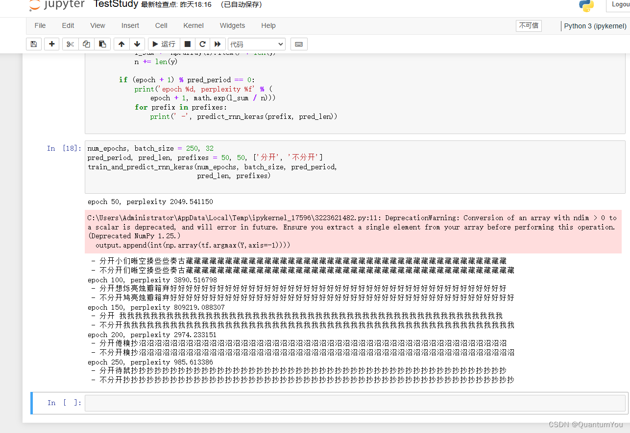
num_epochs, batch_size, lr, clipping_theta = 250, 32, 1e-3, 1e-2 # 注意这里的学习率设置
pred_period, pred_len, prefixes = 50, 50, ['分开', '不分开']
train_and_predict_rnn_pytorch(model, num_hiddens, vocab_size, device,
                            corpus_indices, idx_to_char, char_to_idx,
                            num_epochs, num_steps, lr, clipping_theta,
                            batch_size, pred_period, pred_len, prefixes)

8.3 brief summary

• PyTorch的nn模块提供了循环神经网络层的实现。
• PyTorch的nn.RNN实例在前向计算后会分别返回输出和隐藏状态。该前向计算并不涉及输出层计算。

---

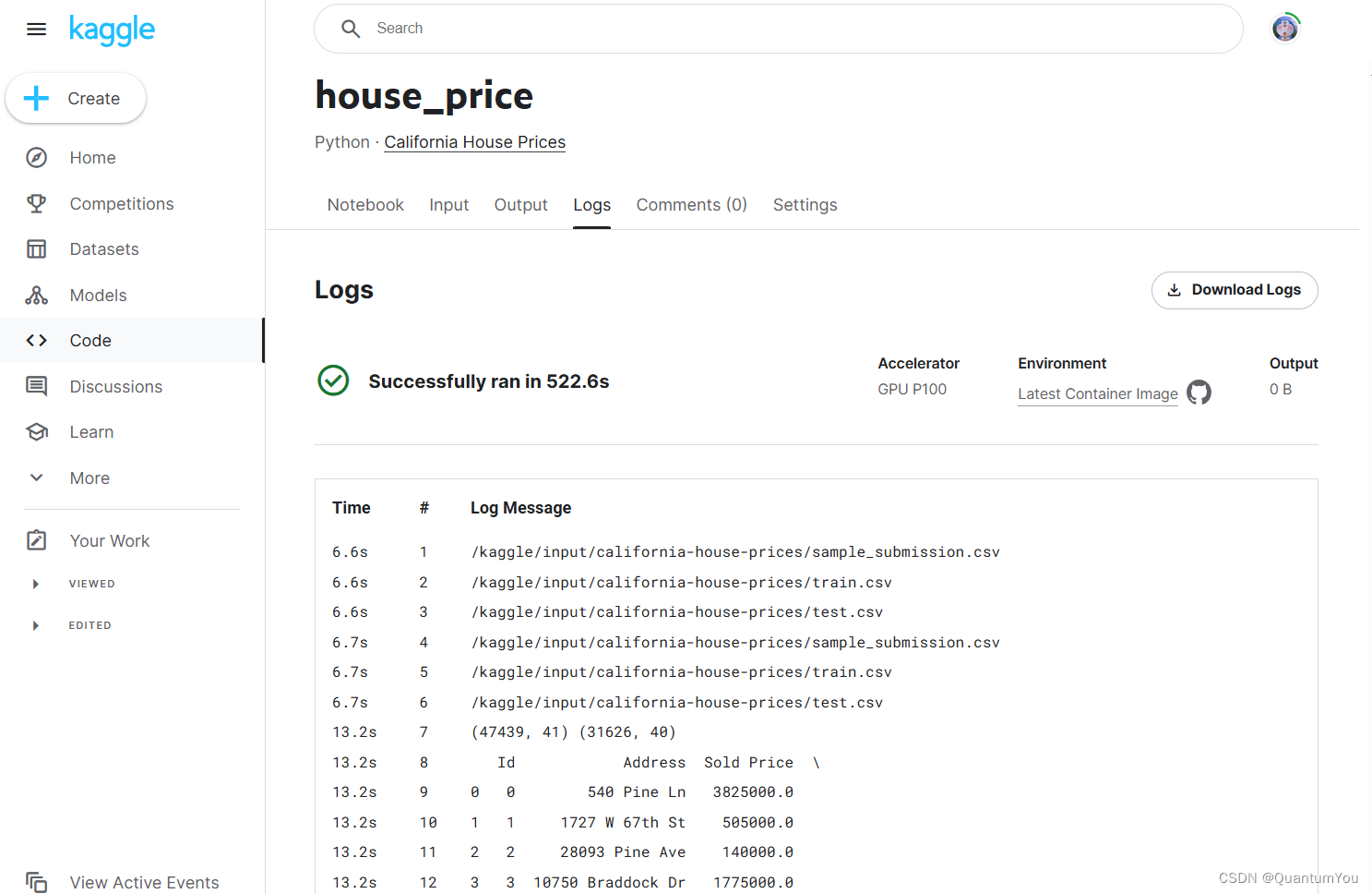
9、Kaggle house_price achieve

9.1 Implement the address

https://www.kaggle.com/competitions/california-house-prices

9.2 Implement screenshots