


Blur detection with OpenCV

Between myself and my father, Jemma, the super-sweet, hyper-active, extra-loving family beagle may be the most photographed dog of all time. Since we got her as a 8-week old puppy, to now, just under three years later, we have accumulated over 6,000+ photos of the dog.
Excessive?
Perhaps. But I love dogs. A lot. Especially beagles. So it should come as no surprise that as a dog owner, I spend a lot of time playing tug-of-war with Jemma’s favorite toys, rolling around on the kitchen floor with her as we roughhouse, and yes, snapping tons of photos of her with my iPhone.
Over this past weekend I sat down and tried to organize the massive amount of photos in iPhoto. Not only was it a huge undertaking, I started to notice a pattern fairly quickly — there were lots of photos with excessive amounts of blurring.
Whether due to sub-par photography skills, trying to keep up with super-active Jemma as she ran around the room, or her spazzing out right as I was about to take the perfect shot, many photos contained a decent amount of blurring.
Now, for the average person I suppose they would have just deleted these blurry photos (or at least moved them to a separate folder) — but as a computer vision scientist, that wasn’t going to happen.
Instead, I opened up an editor and coded up a quick Python script to perform blur detection with OpenCV.
In the rest of this blog post, I’ll show you how to compute the amount of blur in an image using OpenCV, Python, and the Laplacian operator. By the end of this post, you’ll be able to apply the variance of the Laplacian method to your own photos to detect the amount of blurring.
Looking for the source code to this post?
Jump right to the downloads section.
Variance of the Laplacian

Figure 1: Convolving the input image with the Laplacian operator.
My first stop when figuring out how to detect the amount of blur in an image was to read through the excellent survey work, Analysis of focus measure operators for shape-from-focus [2013 Pertuz et al]. Inside their paper, Pertuz et al. reviews nearly 36 different methods to estimate the focus measure of an image.
If you have any background in signal processing, the first method to consider would be computing the Fast Fourier Transform of the image and then examining the distribution of low and high frequencies — if there are a low amount of high frequencies, then the image can be considered blurry. However, defining what is a low number of high frequencies and what is a high number of high frequencies can be quite problematic, often leading to sub-par results.
Instead, wouldn’t it be nice if we could just compute a single floating point value to represent how blurry a given image is?
Pertuz et al. reviews many methods to compute this “blurryness metric”, some of them simple and straightforward using just basic grayscale pixel intensity statistics, others more advanced and feature-based, evaluating the Local Binary Patterns of an image.
After a quick scan of the paper, I came to the implementation that I was looking for: variation of the Laplacian by Pech-Pacheco et al. in their 2000 ICPR paper, Diatom autofocusing in brightfield microscopy: a comparative study.
The method is simple. Straightforward. Has sound reasoning. And can be implemented in only a single line of code:
You simply take a single channel of an image (presumably grayscale) and convolve it with the following 3 x 3 kernel:

Figure 2: The Laplacian kernel.
And then take the variance (i.e. standard deviation squared) of the response.
If the variance falls below a pre-defined threshold, then the image is considered blurry; otherwise, the image is not blurry.
The reason this method works is due to the definition of the Laplacian operator itself, which is used to measure the 2nd derivative of an image. The Laplacian highlights regions of an image containing rapid intensity changes, much like the Sobel and Scharr operators. And, just like these operators, the Laplacian is often used for edge detection. The assumption here is that if an image contains high variance then there is a wide spread of responses, both edge-like and non-edge like, representative of a normal, in-focus image. But if there is very low variance, then there is a tiny spread of responses, indicating there are very little edges in the image. As we know, the more an image is blurred, the less edges there are.
Obviously the trick here is setting the correct threshold which can be quite domain dependent. Too low of a threshold and you’ll incorrectly mark images as blurry when they are not. Too high of a threshold then images that are actually blurry will not be marked as blurry. This method tends to work best in environments where you can compute an acceptable focus measure range and then detect outliers.
Detecting the amount of blur in an image
So now that we’ve reviewed the the method we are going to use to compute a single metric to represent how “blurry” a given image is, let’s take a look at our dataset of the following 12 images:
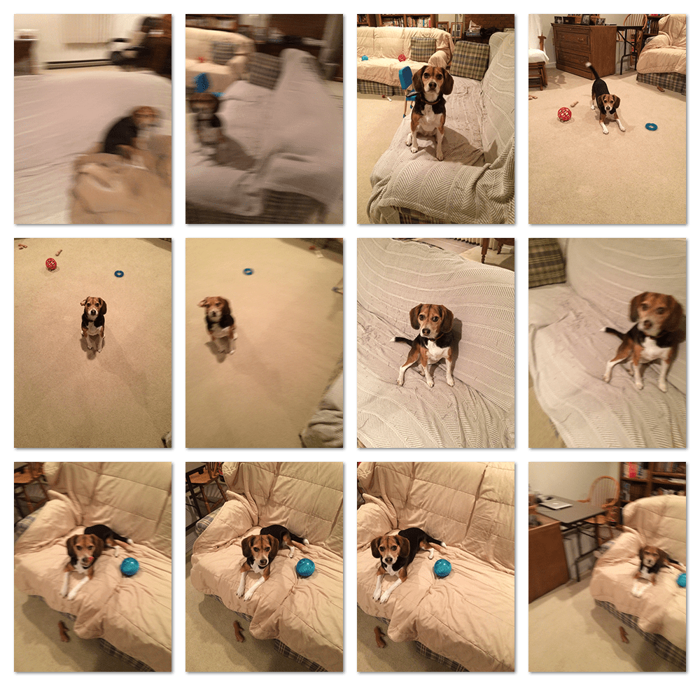
Figure 3: Our dataset of images. Some are blurry, some are not. Our goal is to perform blur detection with OpenCV and mark the images as such.
As you can see, some images are blurry, some images are not. Our goal here is to correctlymark each image as blurry or non-blurry.
With that said, open up a new file, name it detect_blur.py , and let’s get coding:
We start off by importing our necessary packages on Lines 2-4. If you don’t already have myimutils package on your machine, you’ll want to install it now:
From there, we’ll define our variance_of_laplacian function on Line 6. This method will take only a single argument the image (presumed to be a single channel, such as a grayscale image) that we want to compute the focus measure for. From there, Line 9 simply convolves theimage with the 3 x 3 Laplacian operator and returns the variance.
Lines 12-17 handle parsing our command line arguments. The first switch we’ll need is --images , the path to the directory containing our dataset of images we want to test for blurryness.
We’ll also define an optional argument --thresh , which is the threshold we’ll use for the blurry test. If the focus measure for a given image falls below this threshold, we’ll mark the image as blurry. It’s important to note that you’ll likely have to tune this value for your own dataset of images. A value of 100 seemed to work well for my dataset, but this value is quite subjective to the contents of the image(s), so you’ll need to play with this value yourself to obtain optimal results.
Believe it or not, the hard part is done! We just need to write a bit of code to load the image from disk, compute the variance of the Laplacian, and then mark the image as blurry or non-blurry:
We start looping over our directory of images on Line 20. For each of these images we’ll load it from disk, convert it to grayscale, and then apply blur detection using OpenCV (Lines 24-27).
In the case that the focus measure exceeds the threshold supplied a command line argument, we’ll mark the image as “blurry”.
Finally, Lines 35-38 write the text and computed focus measure to the image and display the result to our screen.
Applying blur detection with OpenCV
Now that we have detect_blur.py script coded up, let’s give it a shot. Open up a shell and issue the following command:

Figure 4: Correctly marking the image as “blurry”.
The focus measure of this image is 83.17, falling below our threshold of 100; thus, we correctly mark this image as blurry.

Figure 5: Performing blur detection with OpenCV. This image is marked as “blurry”.
This image has a focus measure of 64.25, also causing us to mark it as “blurry”.

Figure 6: Marking an image as “non-blurry”.
Figure 6 has a very high focus measure score at 1004.14 — orders of magnitude higher than the previous two figures. This image is clearly non-blurry and in-focus.

Figure 7: Applying blur detection with OpenCV and Python.
The only amount of blur in this image comes from Jemma wagging her tail.

Figure 8: Basic blur detection with OpenCV and Python.
The reported focus measure is lower than Figure 7, but we are still able to correctly classify the image as “non-blurry”.

Figure 9: Computing the focus measure of an image.
However, we can clearly see the above image is blurred.

Figure 10: An example of computing the amount of blur in an image.
The large focus measure score indicates that the image is non-blurry.

Figure 11: The subsequent image in the dataset is marked as “blurry”.
However, this image contains dramatic amounts of blur.

Figure 12: Detecting the amount of blur in an image using the variance of Laplacian.

Figure 13: Compared to Figure 12 above, the amount of blur in this image is substantially reduced.

Figure 14: Again, this image is correctly marked as not being “blurred”.
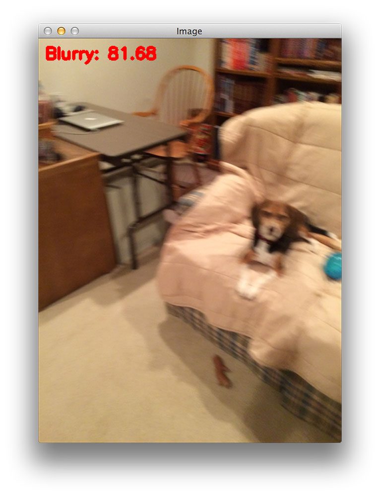
Figure 15: Lastly, we end our example by using blur detection in OpenCV to mark this image as “blurry”.
Summary
In this blog post we learned how to perform blur detection using OpenCV and Python.
We implemented the variance of Laplacian method to give us a single floating point value to represent the “blurryness” of an image. This method is fast, simple, and easy to apply — we simply convolve our input image with the Laplacian operator and compute the variance. If the variance falls below a predefined threshold, we mark the image as “blurry”.
It’s important to note that threshold is a critical parameter to tune correctly and you’ll often need to tune it on a per-dataset basis. Too small of a value, and you’ll accidentally mark images as blurry when they are not. With too large of a threshold, you’ll mark images as non-blurry when in fact they are.
Be sure to download the code using the form at the bottom of this post and give it a try!
Downloads:
Resource Guide (it’s totally free).


 3145
3145

 被折叠的 条评论
为什么被折叠?
被折叠的 条评论
为什么被折叠?
 到【灌水乐园】发言


