三次样条插值（cubic spline Interpolation）笔记

最新推荐文章于 2025-03-07 08:13:52 发布

Shoulderc

最新推荐文章于 2025-03-07 08:13:52 发布

阅读量4.9k

点赞数 45

文章标签：笔记

本文链接：https://blog.csdn.net/Shoulderc/article/details/144059684

版权

文章目录

前言
一、三次样条曲线介绍
二、三次样条曲线推导
- 1. 样条插值原理
- 2. 边界条件
三、c++代码实现
参考文献

前言

本文为在学习三次样条插值时的一些记录，包含原理介绍、公式推导。最后参考github上开源项目的python代码，完成c++实现。

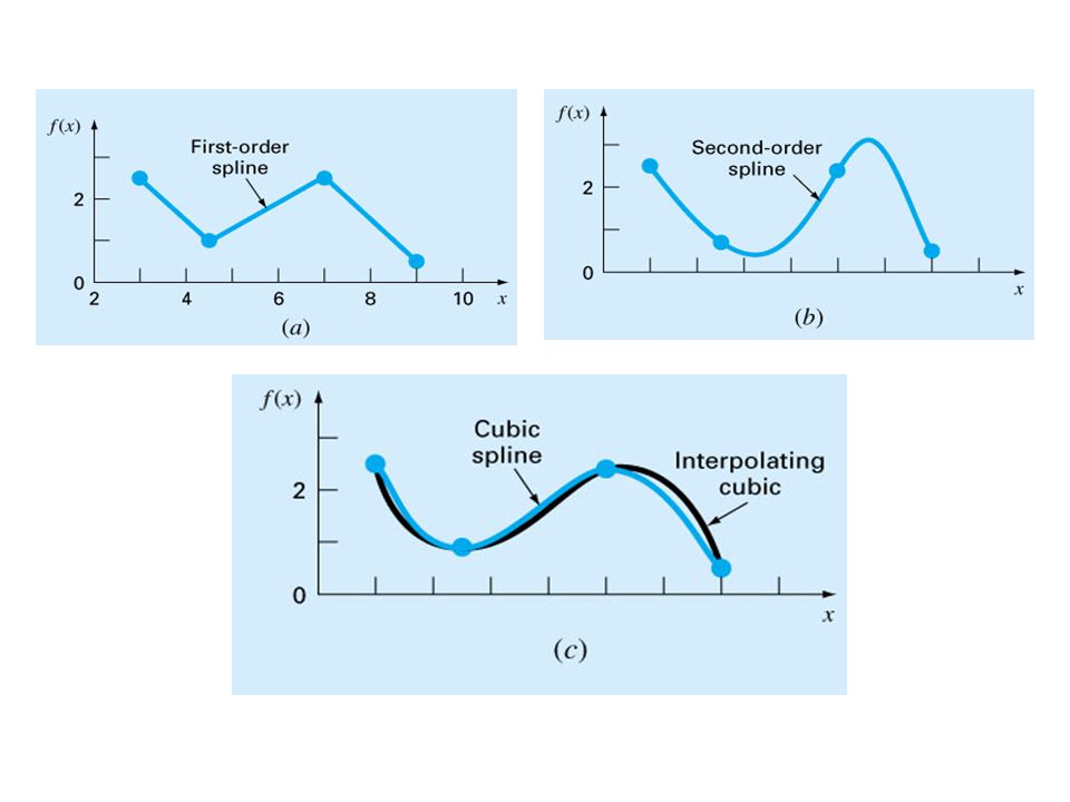
一、三次样条曲线介绍

三次样条插值是一种常用的数学方法，用于在一组已知点的边界内构造新的点。这些新的点是插值函数（称为样条）的函数值，它本身由多个三次分段多项式组成。具体公式如下，
$\begin{gather} f(x)= \left\{\begin{matrix} a_{1}+b_{1}x+c_{1}x^{2}+d_{1}x^3 & x \in [x_{0}, x_{1}] \\ a_{2}+b_{2}x+c_{2}x^{2}+d_{2}x^3 & x \in [x_{1}, x_{2}] \\ \vdots & \\ a_{n}+b_{n}x+c_{n}x^{2}+d_{n}x^3 & x \in [x_{n-1}, x_{n}] \end{matrix}\right. \end{gather}$

其中 $x_{0}, x_{1},...,x_{n}$ 为已知的边界点，每两个边界点的曲线都是一段三次多项式曲线，且这些曲线满足连续、光滑的条件。
图片来源：样条插值(Spline Interpolation)
三次样条曲线的具体定义如下：
在区间 $[a, b]$ 内，对于给定的函数值 $y_{i}=f(x_{i}), i=0, 1,2,...,n$ , 其中 $a=x_{0} < x_{1} <x_{2}<...<x_{n}=b$ 。如果函数 $S (x)$ 满足条件：

$S (x)$ 在每个子区间 $x_{i}, x_{i+1}], i=0, 1,2,...,n-1$ 上都是不高于三次的多项式；
$S(x), S^{'}(x), S^{''}(x)$ 在 $[a, b]$ 上都连续；
$S(x)=y_{i}, i=0, 1,2,...,n$

则称 $S (x)$ 为函数 $f (x)$ 关于点 $x_{0}, x_{1},...,x_{n}$ 的三次样条曲线。

此处函数 $f (x)$ 可写为三次曲线多项式 $f(x)=a+bx+cx^{2}+dx^3$ 。

二、三次样条曲线推导

1. 样条插值原理

样条插值函数的表达式为：
$S_{i}(x)=a_{i}+b_{i}(x-x_{i})+c_{i}(x-x_{i})^{2}+d_{i}(x-x_{i})^{3}$
其中， $\in [x_{i}, x_{i+1}], i=0, 1, 2,...,n-1$
上述样条插值函数包含 $n + 1$ 个边界点， $n + 1$ 个边界点划分成 $n$ 段区间， $n$ 段区间对应 $n$ 个分段三次多项式函数；在每个三次多项式函数中都有4个位置系数 $a, b, c, d$ ，因此样条插值函数共有 $4 n$ 个未知数。
求解样条插值函数的 $4 n$ 个未知数需要 $4 n$ 个方程。
首先根据连续性原则，每个分段函数都经过其两侧端点（已知边界点），因此可得到 $2 n$ 个方程：
$\begin{gather} \begin{matrix} S_{0}(x_{0})=a_{0}+b_{0}(x_{0}-x_{0})+c_{0}(x_{0}-x_{0})^{2}+d_{0}(x_{0}-x_{0})^{3} \\ S_{0}(x_{1})=a_{0}+b_{0}(x_{1}-x_{0})+c_{0}(x_{1}-x_{0})^{2}+d_{0}(x_{1}-x_{0})^{3} \\ S_{1}(x_{1})=a_{1}+b_{1}(x_{1}-x_{1})+c_{1}(x_{1}-x_{1})^{2}+d_{1}(x_{1}-x_{1})^{3} \\ S_{1}(x_{2})=a_{1}+b_{1}(x_{2}-x_{1})+c_{1}(x_{2}-x_{1})^{2}+d_{1}(x_{2}-x_{1})^{3} \\ \vdots \\ S_{n-1}(x_{n-1})=a_{n-1}+b_{n-1}(x_{n-1}-x_{n-1})+c_{n-1}(x_{n-1}-x_{n-1})^{2}+d_{n-1}(x_{n-1}-x_{n-1})^{3} \\ S_{n-1}(x_{n})=a_{n-1}+b_{n-1}(x_{n}-x_{n-1})+c_{n-1}(x_{n}-x_{n-1})^{2}+d_{n-1}(x_{n}-x_{n-1})^{3} \\ \end{matrix} \end{gather}$
由三次样条曲线定义： $S(x)=y_{i}, i=0, 1,2,...,n$ ，结合上述方程可知 $S_{i}(x_{i})=a_{i}=y_{i}$ ，得到：

$\begin{align} a_{i}=y_{i}, i =0,1,2,...,n-1 \end{align}$

定义步长 $h_{i}=x_{i+1}-x_{i}$ ，根据连续性原则，结合上述方程可知 $S_{i}(x_{i+1})=S_{i+1}(x_{i+1})$ ，即：
$\begin{align} a_{i+1}=a_{i}+b_{i}h_{i}+c_{i}h_{i}^{2}+d_{i}h_{i}^{3}, i=0,1,2,...,n-2 \end{align}$
其次，根据光滑性原则，相邻的两个分段函数连接处低阶导数相等，在三次样条函数中，
$\begin{gather} S_{i}^{'}(x_{i+1})=S_{i+1}^{'}(x_{i+1}), i=0,1,2,...,n-2 \\ S_{i}^{''}(x_{i+1})=S_{i+1}^{''}(x_{i+1}), i=0,1,2,...,n-2 \\ \end{gather}$
共 $2 (n - 1)$ 个方程。

由
$\begin{gather} S_{i}^{'}(x)=b_{i} + 2c_{i}(x - x_{i}) + 3d_{i}(x-x_{i})^{2} \\ S_{i}^{''}(x)=2c_{i}+6d_{i}(x-x_{i}) \end{gather}$
结合式(5)、(6)可得：
$\begin{gather} b_{i} + 2c_{i}(x_{i+1} - x_{i}) + 3d_{i}(x_{i+1}-x_{i})^{2}=b_{i+1}, i=0,1,2,...,n-2 \\ 2c_{i}+6d_{i}(x_{i+1}-x_{i})=2c_{i+1}, i=0,1,2,...,n-2 \end{gather}$
将 $h_{i}=x_{i+1}-x_{i}$ 带入上式并化简可得：
$\begin{gather} b_{i} + 2c_{i}h_{i} + 3d_{i}h_{i}^{2}=b_{i+1}, i=0,1,2,...,n-2 \\ c_{i}+3d_{i}h_{i}=c_{i+1}, i=0,1,2,...,n-2 \end{gather}$

令 $m_{i}=c_{i}$ 作为未知变量，并变换式(12)可得：

$\begin{gather} d_{i} =\frac{m_{i+1} - m_{i}} {3h_{i}} \end{gather}$
将式(13)带入式(4)可得：
$\begin{gather} b_{i} =\frac{a_{i+1} - a_{i}} {h_{i}}- \frac{2}{3}m_{i}h_{i}-\frac{1} {3}m_{i+1}h_{i} \end{gather}$
将式(14)、(13)带入(11)可得：
$\begin{gather} h_{i} m_{i}+2(h_{i}+h_{i+1})m_{i+1}+h_{i+1}m_{i+2}=3[\frac{a_{i+2} - a_{i+1}} {h_{i+1}}-\frac{a_{i+1} - a_{i}} {h_{i}}], \quad i=0, 1,2,...,n-2 \end{gather}$
式(15)写成矩阵的形式为：
$\begin{gather} AX=B \end{gather}$
其中：
$\begin{gather*} A= \begin{bmatrix} h_{0} & 2(h_{0}+h_{1}) & h_{1} & 0 & 0 & \cdots & \cdots &0\\ 0 & h_{1} & 2(h_{1}+h_{2}) & h_{2} & 0 & \cdots & \cdots &0 \\ 0 & 0 & h_{2}& 2(h_{2}+h_{3})& h_{3} & \cdots & \cdots & \vdots\\ \vdots & \vdots & 0 & \ddots & \ddots &\ddots & \cdots & \vdots \\ \vdots & \vdots & \vdots & \vdots & \ddots& \ddots& \ddots & \vdots \\ \vdots & \vdots & \vdots & \vdots & \vdots & \ddots & \ddots & 0\\ 0& 0 & \cdots & \cdots & 0 & h_{n-2} & 2(h_{n-2}+h_{n-1}) & h_{n-1} \end{bmatrix} \end{gather*}$

$\begin{gather*} X= \begin{bmatrix} m_{0} & m_{1} & m_{2} & ... & m_{n} \end{bmatrix}^{T} \end{gather*}$

$\begin{gather*} B= 3 \begin{bmatrix} \frac{a_{2}-a_{1}}{h_{1}} - \frac{a_{1}-a_{0}}{h_{0}} \\ \frac{a_{3}-a_{2}}{h_{2}} - \frac{a_{2}-a_{1}}{h_{1}} \\ \vdots \\ \frac{a_{n}-a_{n-1}}{h_{n-1}} - \frac{a_{n-1}-a_{n-2}}{h_{n-1}} \end{bmatrix} \end{gather*}$
上述矩阵方程中，共 $n - 2$ 个等式，包含 $n$ 个未知数，因此还无法求解。

结合三次样条插值的连通性和光滑性，共构造了 $4 (n - 1)$ 个方程，对于包含 $4 n$ 个未知系数的三次样条函数来说，还差2个方程才能求解。剩下的两个方程将有下文的边界条件约束给出。

2. 边界条件

常见的边界条件有：自然边界、固定边界、非节点边界
1、自然边界：指定端点二阶导数为0，即 $S^{''}(x_{0})=0=S^{''}(x_{n})$
$\begin{gather} S^{''}(x_{0})=2m_{0}+6d_{0}(x_{0}-x_{0})=0 \\ S^{''}(x_{n})=2m_{n-1}+6d_{n-1}(x_{n}-x_{n-1})=0 \end{gather}$
由于 $x_{n}>x_{n-1}$ ，可得：
$\begin{gather} m_{0}=m_{n}=0 \end{gather}$
则式(16)的矩阵可改写为：
$\begin{gather*} A= \begin{bmatrix} 1 & 0 & 0 & 0 & 0 & 0 & \cdots & \cdots &0 \\ 0 &h_{0} & 2(h_{0}+h_{1}) & h_{1} & 0 & 0 & \cdots & \cdots &0\\ 0 &0 & h_{1} & 2(h_{1}+h_{2}) & h_{2} & 0 & \cdots & \cdots &0 \\ 0 &0 & 0 & h_{2}& 2(h_{2}+h_{3})& h_{3} & \cdots & \cdots & \vdots\\ 0 &0 & 0 & 0 & \ddots & \ddots &\ddots & \cdots & \vdots \\ \vdots &\vdots & \vdots & \vdots & \vdots & \ddots& \ddots& \ddots & \vdots \\ \vdots &\vdots & \vdots & \vdots & \vdots & \vdots & \ddots & \ddots & 0\\ 0 &0& 0 & \cdots & \cdots & 0 & h_{n-2} & 2(h_{n-2}+h_{n-1}) & h_{n-1} \\ 0 &0& 0 & \cdots & \cdots & 0 & 0 & 0 & 1 \end{bmatrix} \end{gather*}$

$\begin{gather*} X= \begin{bmatrix} m_{0} & m_{1} & m_{2} & ... & m_{n} \end{bmatrix}^{T} \end{gather*}$

$\begin{gather*} B= 3 \begin{bmatrix} 0 \\ \frac{a_{2}-a_{1}}{h_{1}} - \frac{a_{1}-a_{0}}{h_{0}} \\ \frac{a_{3}-a_{2}}{h_{2}} - \frac{a_{2}-a_{1}}{h_{1}} \\ \vdots \\ \frac{a_{n}-a_{n-1}}{h_{n-1}} - \frac{a_{n-1}-a_{n-2}}{h_{n-1}} \\ 0 \end{bmatrix} \end{gather*}$
此时构造出 $n$ 个方程求解 $n$ 个未知数，然后通过 $m$ 与三次多项式系数 $a, b, c, d$ 之间的关系计算出三次样条函数的所有未知数。
2、固定边界：给定两个端点的一阶导数值， $S_{0}^{'}(x_{0})=A, S_{n-1}^{'}(x_{n})=B$ 。结合上文样条插值原理中的公式，可得：
$\begin{gather} 2h_{0}m_{0}+h_{0}m_{1}=3[\frac{a_{1}-a_{0}}{h_{0}}-A] \\ h_{n-1}m_{n-1}+2h_{n-1}m_{n}=3[B-\frac{a_{n}-a_{n-1}}{h_{n-1}}] \end{gather}$
同样的可改写式(16)矩阵方程 $A X = B$ ，然后进行求解。
3、非节点边界：假设第1段和第2段曲线的3阶导在端点处相等，第n-1段和第n段函数的3阶导在端点处相等，即：
$S_{0}^{'''}(x_{0})=S_{1}^{'''}(x_{0}), S_{n-2}^{'''}(x_{n-1})=S_{n-1}^{'''}(x_{n-1})$
结合上文样条插值原理中的公式，可得：
$\begin{gather} -h_{1}m_{0}+(h_{0}+h_{1})m_{1}-h_{0}m_{2}=0 -h_{n-1}m_{n-2}+(h_{n-2}+h_{n-1})m_{n-1}-h_{n-2}m_{n}=0 \end{gather}$
同样的可改写式(16)矩阵方程 $A X = B$ ，然后进行求解。

未知数 $m$ 与三次样条函数系数 $a, b, c, d$ 的关系如下：
$\begin{gather*} a_{i} = y_{i}, \quad i = 0,1,2,...,n\\ b_{i} = \frac{a_{i+1} - a_{i}} {h_{i}}- \frac{2}{3}m_{i}h_{i}-\frac{1} {3}m_{i+1}h_{i}, \quad i = 0,1,2,...,n-1\\ c_{i} = m_{i}, \quad i = 0,1,2,...,n \\ d_{i} = \frac{m_{i+1} - m_{i}} {3h_{i}}, \quad i = 0,1,2,...,n-1 \end{gather*}$
其中， $y_{i}$ 为已知边界点对应的值。

三、c++代码实现

根据文章第二部分的公式推导，采用自然边界条件。参考github上开源库PythonRobotics 中三次样条曲线的python代码，完成c++版本的实现。

cubic_spline.h

/*
 * @FilePath: /CubicSpline/cubic_spline.h
 * @Reference: https://github.com/AtsushiSakai/PythonRobotics
 */
#include <iostream>
#include <vector>
#include <cmath>
#include <algorithm>

#include "Eigen/Dense"
#include "Eigen/Core"


class CubicSpline1D {
    private:
        std::vector<double> x_, y_;
        
        int nx_;

        std::vector<double> h_;

        std::vector<double> a_, b_, c_, d_;

        Eigen::MatrixXd A_, B_;


        void CalA();

        void CalB();

        void SearchIndex(const int x, int *index_x);

    public:
        CubicSpline1D() {};
        ~CubicSpline1D() {};

        void Init(const std::vector<double> & x, const std::vector<double> & y);

        void CalPosition(const double & x, double *pos);

        void Reset() {};

};

cubic_spline.cpp

/*
 * @FilePath: /CubicSpline/cubic_spline.cpp
 * @Reference: https://github.com/AtsushiSakai/PythonRobotics
 */

#include "cubic_spline.h"

template <typename T>
std::vector<T> cs_diff(const std::vector<T>& input) {
    std::vector<T> result;
    for (size_t i = 1; i < input.size(); ++i) {
        result.push_back(input[i] - input[i - 1]);
    }
    return result;
}

template <typename T>
bool cs_hasNegative(const std::vector<T>& vec) {
    return std::find_if(vec.begin(), vec.end(), [](T num) { return num < 0; }) != vec.end();
}


void CubicSpline1D::Init(const std::vector<double> & x, const std::vector<double> & y) {

    h_ = cs_diff(x);
    if (cs_hasNegative(h_)) {
        std::cout << "ERROR: x coordinates must be sorted in ascending order." << std::endl;
    }

    x_ = x;
    y_ = y;
    nx_ = x.size();

    a_ = y;

    CalA();
    CalB();

    Eigen::MatrixXd c = A_.inverse() * B_;
    // std::vector<double> c_vec(c.col(0).data(), c.col(0).data() + c.col(0).size());
    std::vector<double> c_vec;

    for (int i = 0; i < c.rows(); ++i) {
        for (int j = 0; j < c.cols(); ++j) {
            c_vec.push_back(c(i, j));
        }
    }

    c_ = c_vec;

    double b_i, d_i;
    for (int i = 0; i < nx_ - 1; ++i) {
        d_i = (c_[i+1] - c_[i]) / h_[i] / 3.0;
        b_i = 1.0 / h_[i] * (a_[i+1] - a_[i]) - h_[i] / 3.0 * (2.0 * c_[i] + c_[i + 1]);
        // d_i = i;
        // b_i = i;
        d_.push_back(d_i);
        b_.push_back(b_i);
    }
}

void CubicSpline1D::CalA() {
    A_ = Eigen::MatrixXd::Zero(nx_, nx_);

    A_(0, 0) = 1.0;

    for (int i = 0; i < nx_ - 1; ++i) {
        if (i != nx_ - 2) {
            A_(i+1, i+1) = 2.0 * (h_[i] + h_[i + 1]);
        }
        A_(i + 1, i) = h_[i];
        A_(i, i + 1) = h_[i];
    }

    A_(0, 1) = 0.1;
    A_(nx_ - 1, nx_ - 2) = 0.0;
    A_(nx_ - 1, nx_ - 1) = 1.0;

}

void CubicSpline1D::CalB() {
    B_ = Eigen::MatrixXd::Zero(nx_, 1);

    // h_[i] = 0 ?
    for (int i = 0; i < nx_ -2; ++i) {
        B_(i+1) = 3.0 * (a_[i+2] - a_[i+1]) / h_[i+1] - 
                  3.0 * (a_[i+1] - a_[i]) / h_[i];
    }
}

void BisectRight(const std::vector<double> & a, const double & x, int * index) {
    int hi = a.size();
    double lo = 0.0;
    int mid;
    
    while (lo < hi) {
       mid = std::floor((lo + hi) / 2);
       if (x < a[mid]) {
            hi = mid;
       } else {
            lo = mid + 1;
       }
    }

    *index = lo;
}

void CubicSpline1D::SearchIndex(const int x, int *index_x) {
    int index;
    BisectRight(x_, x, &index);
    *index_x = index - 1;
}

void CubicSpline1D::CalPosition(const double & x, double *pos) {
    
    if (x < x_[0] || x > x_[x_.size() - 1]) {
        std::cout << "ERROR: x is outside the data point's x range." << std::endl;
        return;
    }

    int index = 0;
    SearchIndex(x, &index);

    double dx = x - x_[index];

    double position = a_[index] + b_[index] * dx + c_[index] * dx * dx + 
                      d_[index] * std::pow(dx, 3);
    // double position = 1.0;
    
    *pos = position;

}

main.cpp

/*
 * @FilePath: /CubicSpline/main.cpp
 * @Reference: https://github.com/AtsushiSakai/PythonRobotics
 */


#include "cubic_spline.h"

#include <iostream>
#include <vector>

#include "../../matplotlib-cpp/matplotlibcpp.h"

namespace plt = matplotlibcpp;

int main() {
    std::vector<double> x, y;
    x = {0.0, 1.0, 2.0, 3.0, 4.0};
    y = {1.7, -6.0, 5.0, 6.5, 0.0};
    CubicSpline1D cs1d;
    cs1d.Init(x, y);
    std::vector<double> xi, yi;
    double step = 0.1;
    double pos = 0.0;
    for(double i = 0.0; i < 4.0; i += step) {
        cs1d.CalPosition(i, &pos);
        xi.push_back(i);
        yi.push_back(pos);
    }      

    plt::plot(x, y, "kd");
    plt::plot(xi, yi, "g");
    plt::show();

    return 0;
}

CMakeLists.txt

cmake_minimum_required(VERSION 3.0)

project(my_test)

find_package(Eigen3 3.3 REQUIRED NO_MODULE)
find_package(PythonLibs 3 REQUIRED)

include_directories(${PYTHON_INCLUDE_DIRS})
include_directories(${PROJECT_SOURCE_DIR}/../../matplotlib-cpp)

add_executable(test_cub main.cpp cubic_spline.cpp)

target_link_libraries(test_cub Eigen3::Eigen)
target_link_libraries(test_cub ${PYTHON_LIBRARIES})