


一、朴素贝叶斯核心思想
首先我将举个例子以便理解。假设我收到一封邮件,内容描述如下:您提交的3215号工单:来自李先生的留言。请点击链接查看工单处理进度:https://tingyun.kf5.com/hc/request……
已知在垃圾邮件中经常出现“链接”,“点击”这种单词,我收到的该邮件中包含了这些单词,这个邮件很可能是垃圾邮件。垃圾邮件分类属于监督学习范畴,监督学习指给定一个数据和标签,前提是手中有大量邮件数据,即知道哪些是垃圾邮件哪些不是。
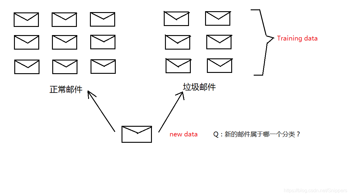
分别计算出邮件中的单词在正常邮件和垃圾邮件中的概率:
P(垃圾|邮件内容) = 一封邮件为垃圾的概率
P(正常|邮件内容) = 一封邮件为正常的概率
如果 P(垃圾|邮件内容) > P(正常|邮件内容),则推测此邮件为垃圾邮件;如果 P(垃圾|邮件内容) < P(正常|邮件内容),则推测此邮件为正常邮件。
二、贝叶斯定理
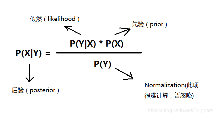
现有一封邮件内容为:“购买 物品, 不是 广告”,如何判断是正常邮件还是垃圾邮件呢?
推导过程如下,需要使用条件独立假设简化
:P(正常|邮件内容) = P(邮件内容|正常)*P(正常)/P(邮件内容)
=P("购买",“物品”,“不是”,“广告”|正常)*P(正常)/P(邮件内容)
=P(“购买”|正常)*P(“物品”|正常)*P(“不是”|正常)*P(“广告”|正常)*P(正常)/P(邮件内容)
=(1/80*1/60*1/60*1/48*2/3 )/P(邮件内容)
P(垃圾|邮件内容) = P(邮件内容|垃圾)*P(垃圾)/P(邮件内容)
=(7/120*1/30*1/40*1/30*1/3 )/P(邮件内容)
垃圾邮件和正常邮件概率的分母均为P(邮件内容),可忽略此项。
如何处理概率为零的情况,样本在测试数据中未出现的状况可能发生,处理方法是使用平滑(smoothy)的思想,例如Add-one smoothy,即在分子加一分母加上词库大小。
应用实例:
# 读取spam.csv文件
import pandas as pd
df = pd.read_csv("data_spam/spam.csv", encoding='latin')
df.head()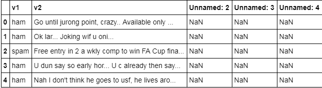
# 重命名数据中的v1和v2列,使得拥有更好的可读性
df.rename(columns={'v1':'Label', 'v2':'Text'}, inplace=True)
df.head() 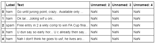
# 把'ham'和'spam'标签重新命名为数字0和1
df['numLabel'] = df['Label'].map({'ham':0, 'spam':1})
df.head() 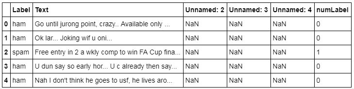
# 统计有多少个ham,有多少个spam
print ("# of ham : ", len(df[df.numLabel == 0]), " # of spam: ", len(df[df.numLabel == 1]))
print ("# of total samples: ", len(df))
# of ham : 4825 # of spam: 747 # of total samples: 5572
# 统计文本的长度信息
text_lengths = [len(df.loc[i,'Text']) for i in range(len(df))]
print ("the minimum length is: ", min(text_lengths))

import numpy as np
import matplotlib.mlab as mlab
import matplotlib.pyplot as plt

plt.hist(text_lengths, 100, facecolor='blue', alpha=0.5)
plt.xlim([0,200])
plt.show()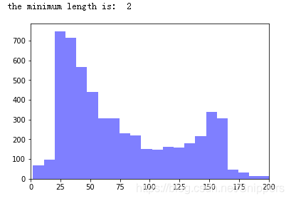
# 导入英文呢的停用词库
from nltk.corpus import stopwords
from sklearn.feature_extraction.text import CountVectorizer
# what is stop wordS? he she the an a that this ...
stopset = set(stopwords.words("english"))

# 构建文本的向量 (基于词频的表示)
#vectorizer = CountVectorizer(stop_words=stopset,binary=True)
vectorizer = CountVectorizer()

# sparse matrix
X = vectorizer.fit_transform(df.Text)
y = df.numLabel
# 把数据分成训练数据和测试数据
from sklearn.model_selection import train_test_split
X_train, X_test, y_train, y_test = train_test_split(X, y, test_size=0.20, random_state=100)
print ("训练数据中的样本个数: ", X_train.shape[0], "测试数据中的样本个数: ", X_test.shape[0])训练数据中的样本个数: 4457 测试数据中的样本个数: 1115
# 利用朴素贝叶斯做训练
from sklearn.naive_bayes import MultinomialNB
from sklearn.metrics import accuracy_score


clf = MultinomialNB(alpha=1.0, fit_prior=True)
clf.fit(X_train, y_train)
y_pred = clf.predict(X_test)
print("accuracy on test data: ", accuracy_score(y_test, y_pred))

# 打印混淆矩阵
from sklearn.metrics import confusion_matrix
confusion_matrix(y_test, y_pred, labels=[0, 1])
accuracy on test data: 0.97847533632287
array([[956, 14],
[ 10, 135]])
——《贪心学院特训营》第四期学习笔记


 8240
8240


 被折叠的 条评论
为什么被折叠?
被折叠的 条评论
为什么被折叠?
 到【灌水乐园】发言


